A gantt chart is a type of chart that shows the start and end times of various tasks.
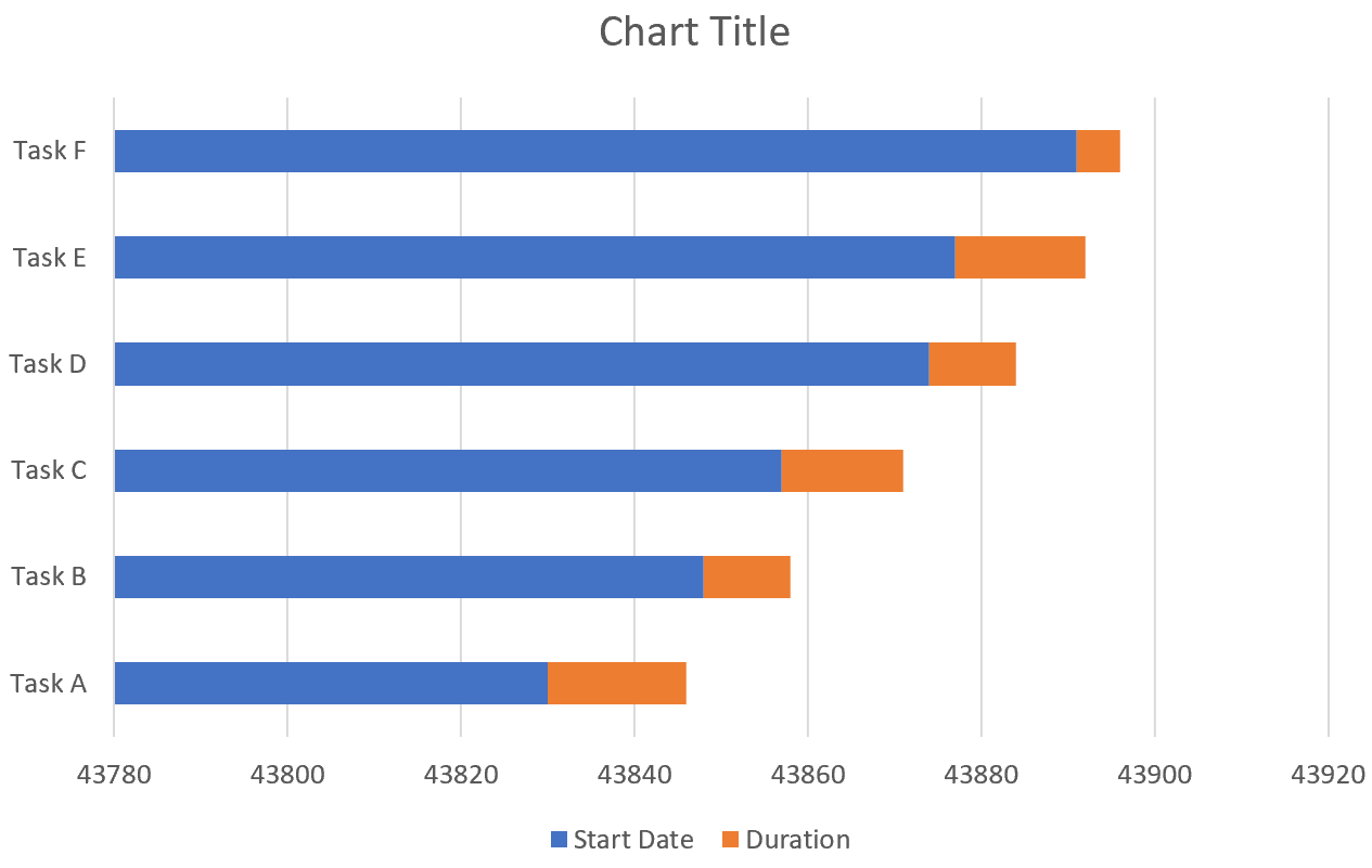
This tutorial explains how to create the following gantt chart in Excel:
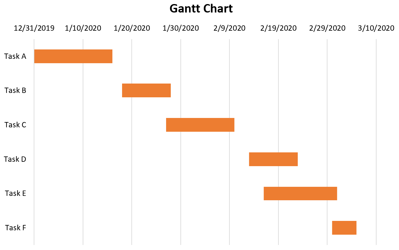
Example: Gantt Chart in Excel
Use the following steps to create a gantt chart in Excel.
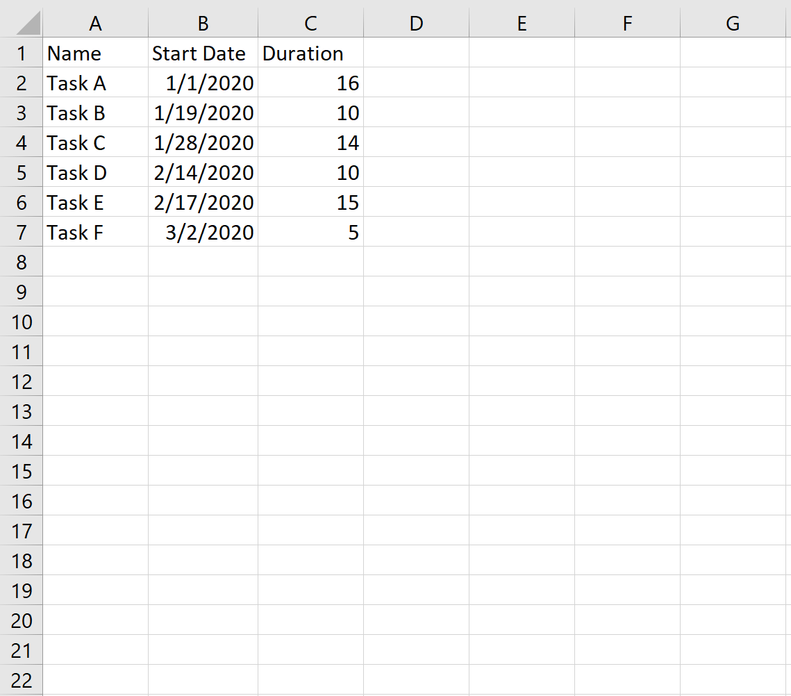
Step 1: Enter the data.
Enter the name, start date, and duration of each task in separate columns:
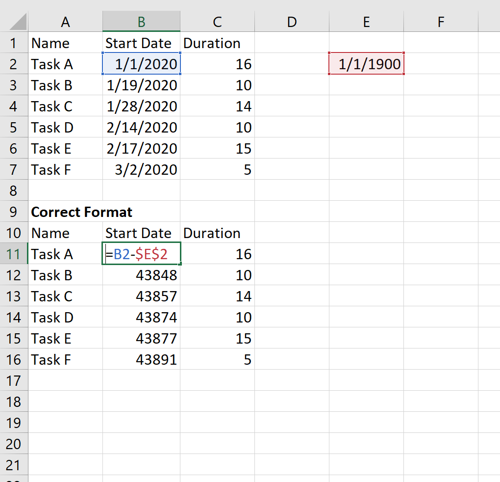
Step 2: Convert the date format to the number of days since Jan. 1, 1990.
By default, dates in Excel are stored as the number of days since Jan 1, 1990. In order to create our gantt chart, we’ll need to convert the dates to numbers using the following formula:
Step 3: Insert a stacked bar chart.
Next, highlight cells A10:C16. In the Charts group within the Insert tab, click on the option that says 2-D stacked bar chart:
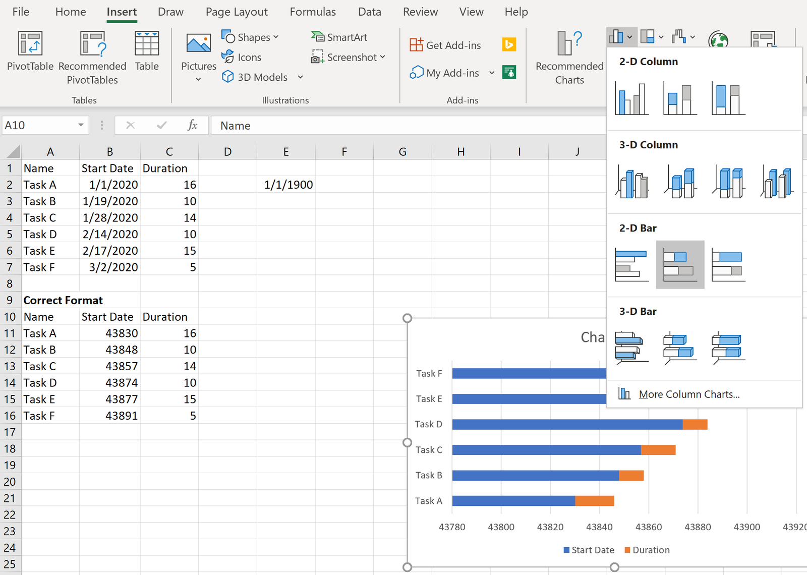
The following chart will automatically appear:
Step 4: Modify the appearance of the chart.
Lastly, we will modify the appearance of the gantt chart.
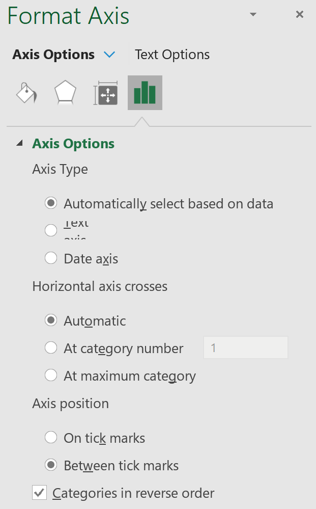
Reverse the order of the tasks.
- Right click any task on the chart. Then click Format Axis…
- Check the box next to Categories in reverse order.
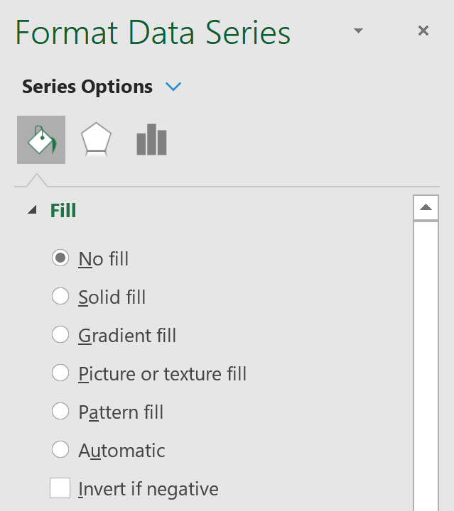
Remove the blue bars.
- Right click on any of the blue bars. Then click Format Data Series…
- Click the paint bucket icon, then Fill, then No fill.
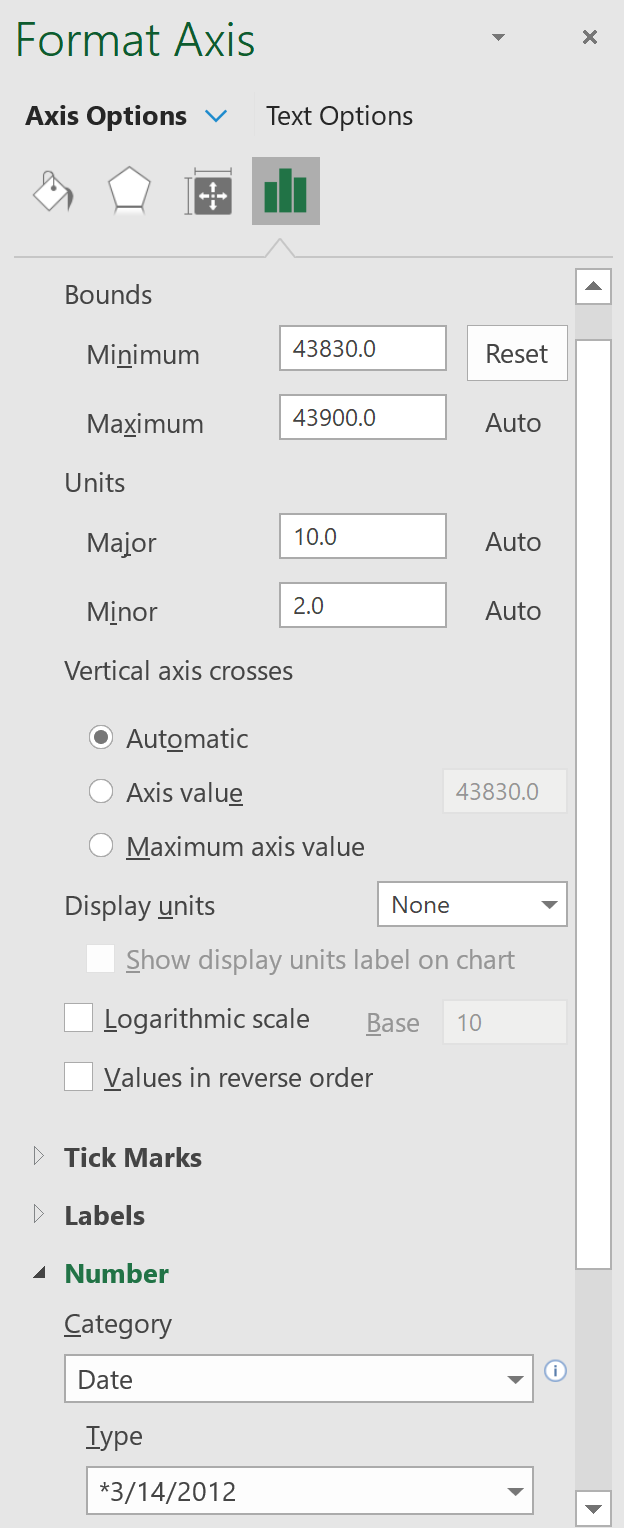
Modify the dates on the x-axis.
- Right click on any of the dates. Then click Format Axis…
- Under Axis Options, change the Minimum value to 43830 to reflect the earliest date of the first task.
- Under Number, change the Category to Date.
Change the title of the chart to anything you’d like. Click on the legend at the bottom and delete it.
The final result should look like this: