You can use the following syntax to filter cells that are arranged horizontally in Excel:
=FILTER(B1:G4, B2:G2 = "value")
This particular formula will return the columns in the range B1:G4 where the cells in the range B2:G2 are equal to “value.”
The following examples show how to use this syntax with the following dataset in Excel:
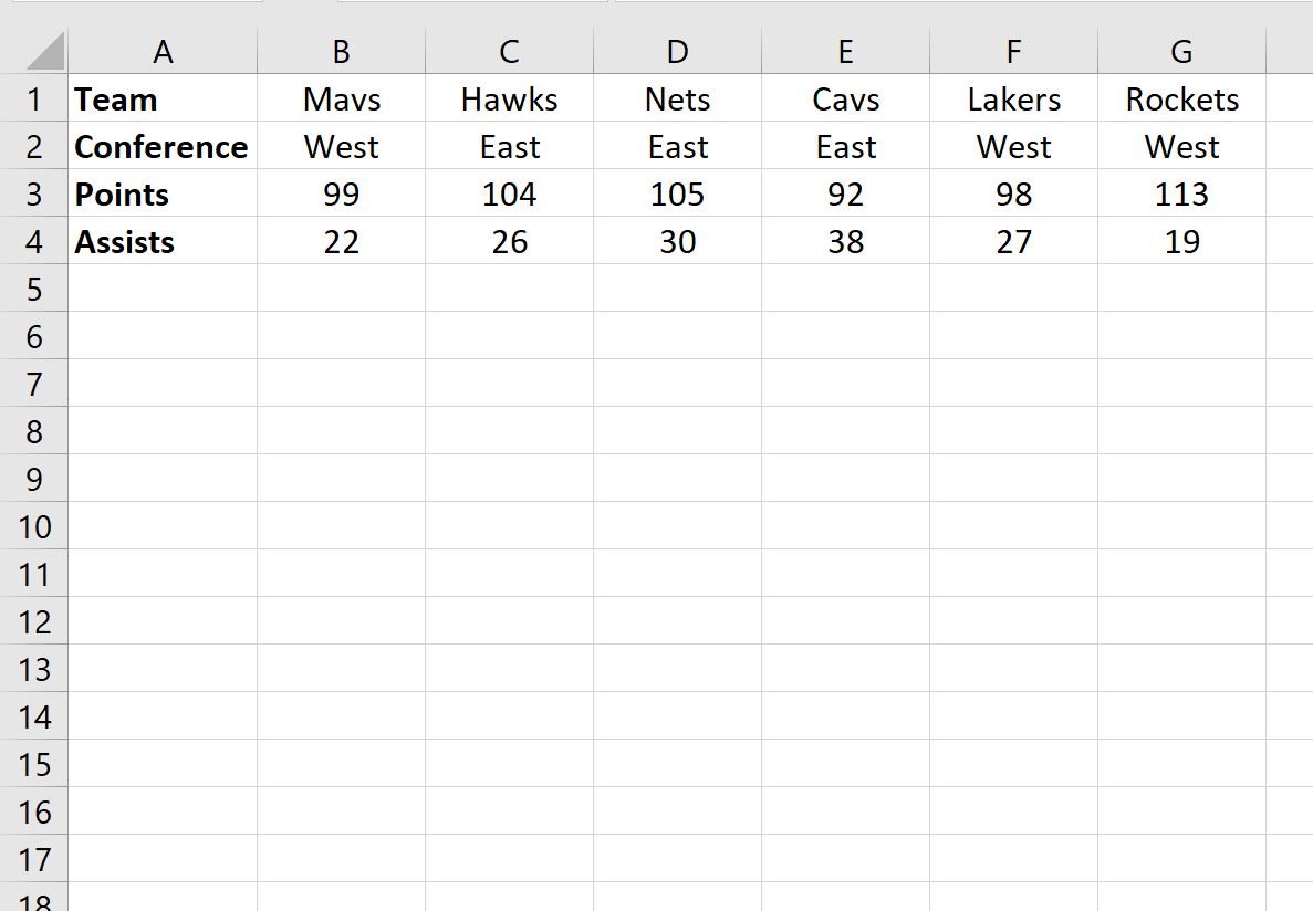
Example 1: Filter Data Horizontally Based on String
We can type the following formula into cell B8 to filter the data to only show columns where the value in the Conference row is equal to “West”:
=FILTER(B1:G4, B2:G2 = "West")
The following screenshot shows how to use this formula in practice:
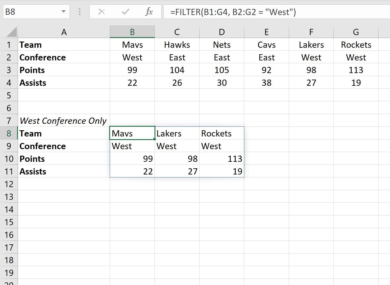
Notice that only the columns that contain “West” in the Conference row are returned.
Example 2: Filter Data Horizontally Based on Numeric Value
We can type the following formula into cell B8 to filter the data to only show columns where the value in the Points row is greater than 100:
=FILTER(B1:G4, B3:G3 > 100)
The following screenshot shows how to use this formula in practice:

Notice that only the columns with a value greater than 100 in the Points row are returned.
Additional Resources
The following tutorials explain how to perform other common tasks in Excel:
Excel: How to Delete Rows with Specific Text
Excel: How to Check if Cell Contains Partial Text
Excel: How to Check if Cell Contains Text from List