How to Perform Exploratory Data Analysis in Python | Online Statistics library

One of the first steps of any data analysis project is exploratory data analysis.

This involves exploring a dataset in three ways:

1. Summarizing a dataset using descriptive statistics.

2. Visualizing a dataset using charts.

3. Identifying missing values.

By performing these three actions, you can gain an understanding of how the values in a dataset are distributed and detect any problematic values before proceeding to perform a hypothesis test or perform statistical modeling.

The following step-by-step example shows how to perform exploratory data analysis for a dataset in Python.

Step 1: Create the Data

First, let’s create the following pandas DataFrame:

import pandas as pd
import numpy as np

#create DataFrame
df = pd.DataFrame({'team': ['A', 'A', 'A', 'A', 'B', 'B', 'B', 'B'],
                   'points': [18, 22, 19, 14, 14, 11, 20, 28],
                   'assists': [5, 7, 7, 9, 12, 9, 9, 4],
                   'rebounds': [11, 8, 10, 6, 6, np.nan, 9, 12]})

We can take a look at the first five rows of the DataFrame by using the head() function:

#view first five rows of dataset
df.head()

	team	points	assists	rebounds
0	A	18	5	11.0
1	A	22	7	8.0
2	A	19	7	10.0
3	A	14	9	6.0
4	B	14	12	6.0

Step 2: Summarize the Data

We can use the describe() function to quickly summarize each numerical variable in the dataset:

#summarize numerical variables
df.describe()

           points	assists 	rebounds
count	8.0000000	8.00000 	7.000000
mean	18.250000	7.75000 	8.857143
std	5.3652320	2.54951 	2.340126
min	11.000000	4.00000 	6.000000
25%	14.000000	6.50000 	7.000000
50%	18.500000	8.00000 	9.000000
75%	20.500000	9.00000 	10.50000
max	28.000000	12.0000         12.00000

For each of the numeric variables we can see the following information:

count: Total number of non-missing values
std: The mean value
min: The minimum value
25%: The value of the first quartile (25th percentile)
50%: The median value (50th percentile)
75%: The value of the third quartile (75th percentile)
max: The maximum value

For the categorical variables in the dataset, we can use value_counts to get a frequency count of each value:

#display frequency counts for team variable
df['team'].value_counts()

A    4
B    4
Name: team, dtype: int64

From the output we can see:

A: This value occurs 4 times.
B: This value occurs 4 times.

We can use the shape function to get the dimensions of the DataFrame in terms of number of rows and number of columns:

#display rows and columns
df.shape

(8, 4)

We can see that the DataFrame has 8 rows and 4 columns.

Step 3: Visualize the Data

We can also create charts to visualize the values in the dataset.

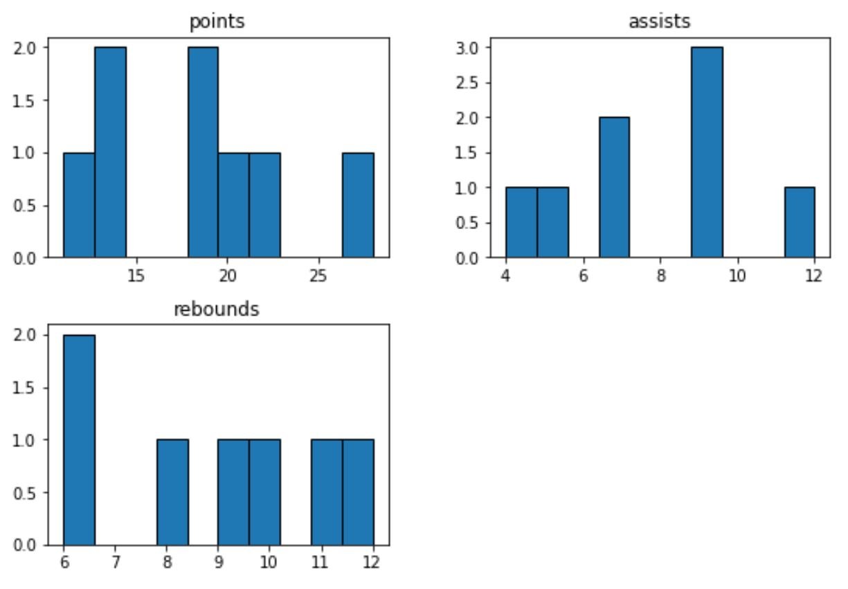
For example, we can use the pandas hist() function to create a histogram of the values for each numerical variable:

#create histogram for each numerical variable
df.hist(grid=False, edgecolor='black')

The x-axis of each histogram shows the values for each variable and the y-axis shows the frequency of each value.

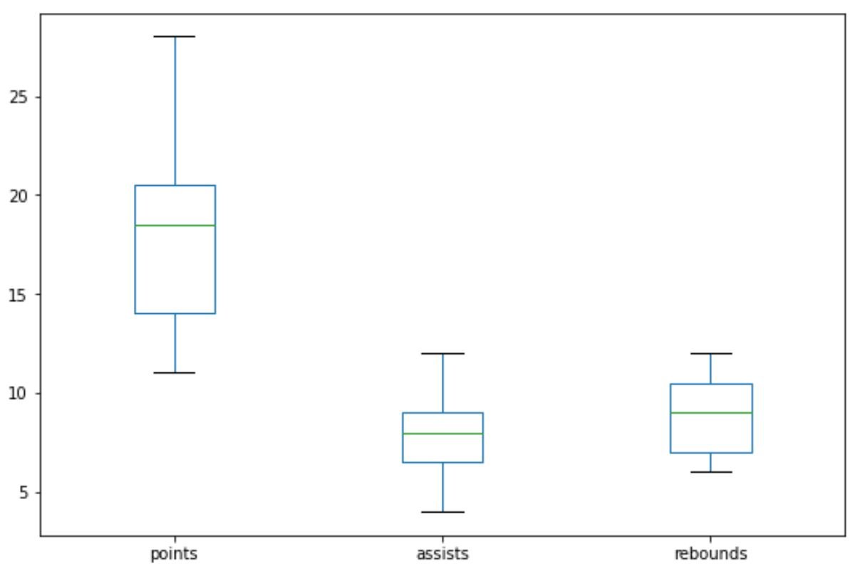
We can also use the pandas boxplot() function to create a boxplot for each numerical variable:

#create boxplot for each numerical variable
df.boxplot(grid=False)

We can also use the geom_boxplot() function to create a boxplot of one variable grouped by another variable:

We can also use the pandas corr() function to create a correlation matrix to view the correlation coefficient between each pairwise combination of numeric variables in the DataFrame:

#create correlation matrix
df.corr()

          points	  assists	 rebounds
points	 1.000000	-0.725841	 0.767007
assists	-0.725841	 1.000000	-0.882046
rebounds 0.767007	-0.882046	 1.000000

Step 4: Identify Missing Values

We can use the following code to count the total number of missing values in each column of the DataFrame:

#count total missing values in each column
df.isnull().sum()

team        0
points      0
assists     0
rebounds    1
dtype: int64

From the output we can see that there is only one missing value in the rebounds column.

All other columns have no missing values.

We have now completed a basic exploratory data analysis on this dataset and have a good understanding of how the values are distributed for each variable in this dataset.

Additional Resources

The following tutorials explain how to perform other common tasks in Python:

How to Create Frequency Tables in Python
How to Create Boxplot from Pandas DataFrame
How to Create a Histogram from Pandas DataFrame