The following step-by-step example shows how to calculate a weighted average within a pivot table in Excel.
Step 1: Enter the Data
First, let’s enter the following dataset that contains information about basketball players on two different teams:

Step 2: Create Helper Column
Suppose we would like to create a pivot table that summarizes the sum of games for each team along with the average points scored per player on each team.
To calculate the average points scored per player, we will need to use a weighted average that takes into account the average points along with the total games.
Since pivot tables in Excel don’t allow you to calculate weighted averages, we will need to first create a helper column in our original dataset.
We can type the following formula into cell E2:
=C2*D2
We can then drag and fill this formula down to the remaining cells in column E:

Step 3: Create the Pivot Table
To create the pivot table, we’ll highlight the cells in the range A1:E9, then click the PivotTable icon within the Insert tab along the top ribbon.
In the PivotTable fields panel that appears, we’ll drag Team to the rows box and Games to the Values box:

The following pivot table will appear:

Step 4: Add Weighted Average Column to Pivot Table
To add a weighted average column that shows the average points per game per player for each team, click any cell in the pivot table, then click the icon called Fields, Items, & Sets within the PivotTable Analyze tab, then click Calculated Field:

In the new window that appears, type = Helper / Games in the Formula box, then click OK:

A new column that shows the average points per game per player for each team will be added to the pivot table:
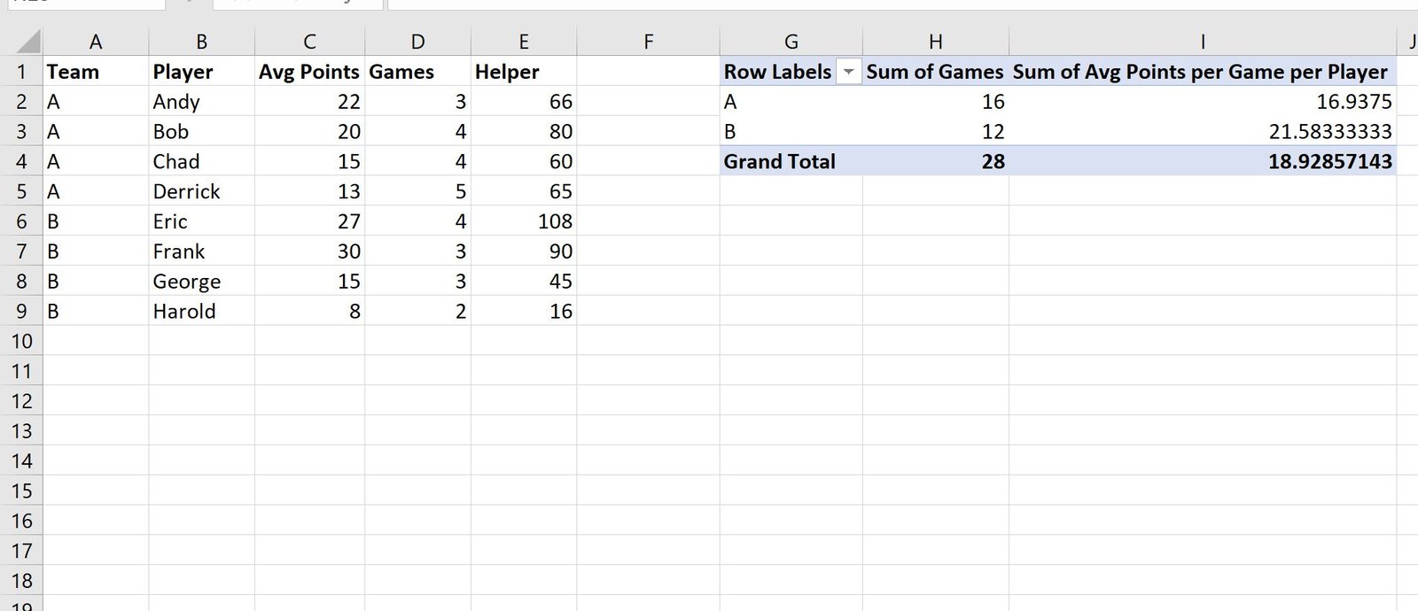
We can confirm that the average points per game per player is correct by manually calculating it from the original dataset.
For example, we could calculate the average points per game per player for team A as:
Avg Points per Game per Player: (22*3 + 20*4 + 15*4 + 13*5) / (3+4+4+5) = 16.9375
This matches the value that appears in the pivot table.
Additional Resources
The following tutorials explain how to perform other common tasks in Excel:
How to Create Tables in Excel
How to Group Values in Pivot Table by Range in Excel
How to Group by Month and Year in Pivot Table in Excel