The following step-by-step example shows how to sum two columns in a pivot table in Excel.
Step 1: Enter the Data
First, let’s enter the following data for three different sales teams:

Step 2: Create the Pivot Table
To create a pivot table, click the Insert tab along the top ribbon and then click the PivotTable icon:

In the new window that appears, choose A1:C16 as the range and choose to place the pivot table in cell E1 of the existing worksheet:

Once you click OK, a new PivotTable Fields panel will appear on the right side of the screen.
Drag the Team field to the Rows box and drag the Sales and Returns fields to the Values box:

The pivot table will automatically be populated with the following values:

Step 3: Sum Two Columns in the Pivot Table
Suppose we would like to create a new column in the pivot table that displays the sum of the Sum of Sales and Sum of Returns columns.
To do so, we need to add a calculated field to the pivot table by clicking on any value in the pivot table, then clicking the PivotTable Analyze tab, then clicking Fields, Items & Sets, then Calculated Field:

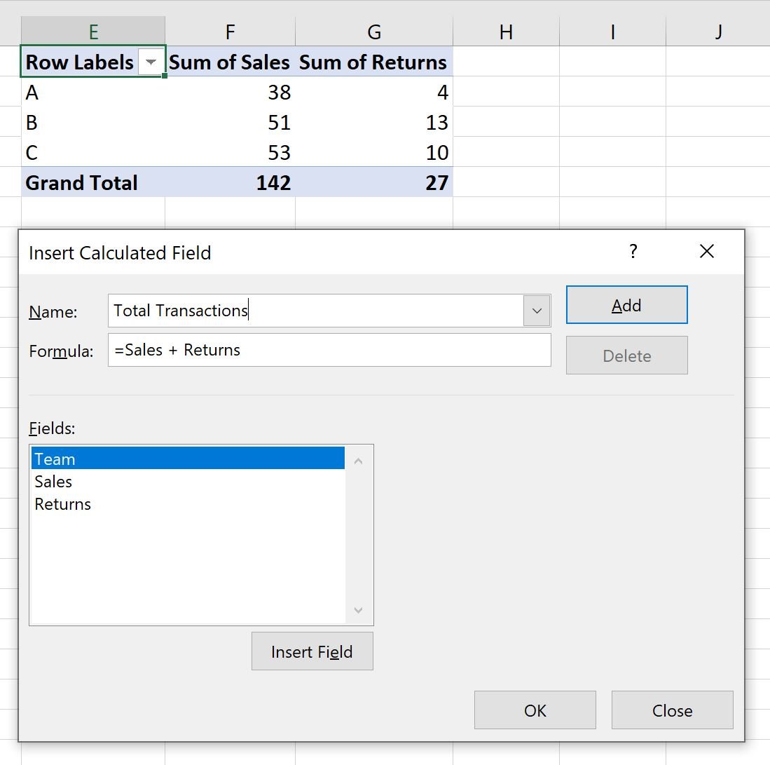
In the new window that appears, type “Total Transactions” in the Name field, then type = Sales + Returns in the Formula field.
Then click Add, then click OK.
This calculated field will automatically be added to the pivot table:

This new field displays the sum of the Sum of Sales and Sum of Returns for each sales team.
Additional Resources
The following tutorials explain how to perform other common tasks in Excel:
How to Create Tables in Excel
How to Group Values in Pivot Table by Range in Excel
How to Group by Month and Year in Pivot Table in Excel