Often you may want to calculate the sum and the count of the same field in a pivot table in Excel.
You can easily do this by dragging the same field into the Values box twice when creating a pivot table.
The following example shows exactly how to do so.
Example: Calculate Sum & Count of Same Field in Excel Pivot Table
Suppose we have the following dataset in Excel that shows the sales of various products:

Now suppose we insert the following pivot table to summarize the sum of sales by product:

Now suppose we would also like to summarize the count of sales for each product.
To do so, we can simply drag the Sales value in the PivotTable Fields panel to the Values box again:

Next, click on the dropdown arrow next to Sum of Sales2 and click on Value Field Settings:

In the new window that appears, click Count and then click OK:

A new field will be added to the pivot table that shows the count of sales:

Feel free to click on the new field name and change the name to “Count of Sales”:
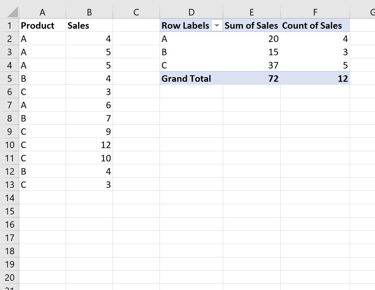
The pivot table now shows the sum of sales and the count of sales for each product.
Additional Resources
The following tutorials explain how to perform other common operations in Excel:
Excel: How to Filter Top 10 Values in Pivot Table
Excel: How to Sort Pivot Table by Grand Total
Excel: How to Calculate the Difference Between Two Pivot Tables