The following step-by-step example shows how to calculate the percentage difference between two columns in a pivot table in Excel.
Step 1: Enter the Data
First, let’s enter the following sales data for three different stores:

Step 2: Create the Pivot Table
Next, let’s create the following pivot table to summarize the total sales by store and by year:

Step 3: Calculate Percentage Difference Between Two Columns in the Pivot Table
Suppose we would like to create a new column in the pivot table that displays the percentage difference between the Sum of 2021 and Sum of 2022 columns.
To do so, we need to add a calculated field to the pivot table by clicking on any value in the pivot table, then clicking the PivotTable Analyze tab, then clicking Fields, Items & Sets, then Calculated Field:

In the new window that appears, type “Percentage Difference” in the Name field, then type the following in the Formula field:
= ('2022' - '2021') / '2021'
Then click Add, then click OK.

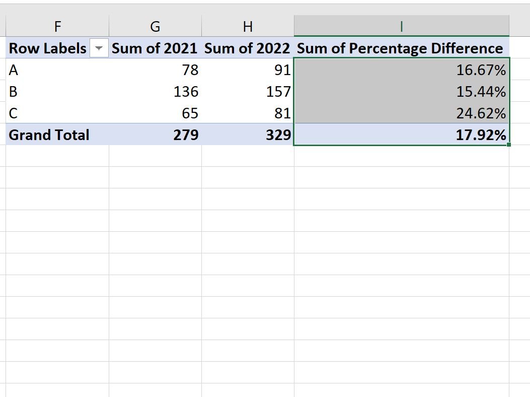
This calculated field will automatically be added to the pivot table:

This new field displays the percentage difference between the 2022 and 2021 sales for each store.
For example:
- There was a 16.67% increase in sales between 2021 and 2022 for store A.
- There was a 15.44% increase in sales between 2021 and 2022 for store B.
- There was a 24.62% increase in sales between 2021 and 2022 for store C.
Feel free to highlight the values in the new field and change their format to a percentage format:
Additional Resources
The following tutorials explain how to perform other common tasks in Excel:
How to Sum Two Columns in a Pivot Table in Excel
How to Subtract Two Columns in a Pivot Table in Excel
How to Calculate Weighted Average in a Pivot Table in Excel