Often you may want to filter values in a pivot table in Excel using a “Greater Than” filter.
Fortunately this is easy to do using the Value Filters dropdown menu within the Row Labels column of a pivot table.
The following example shows exactly how to do so.
Example: Filter Data in Pivot Table Using “Greater Than”
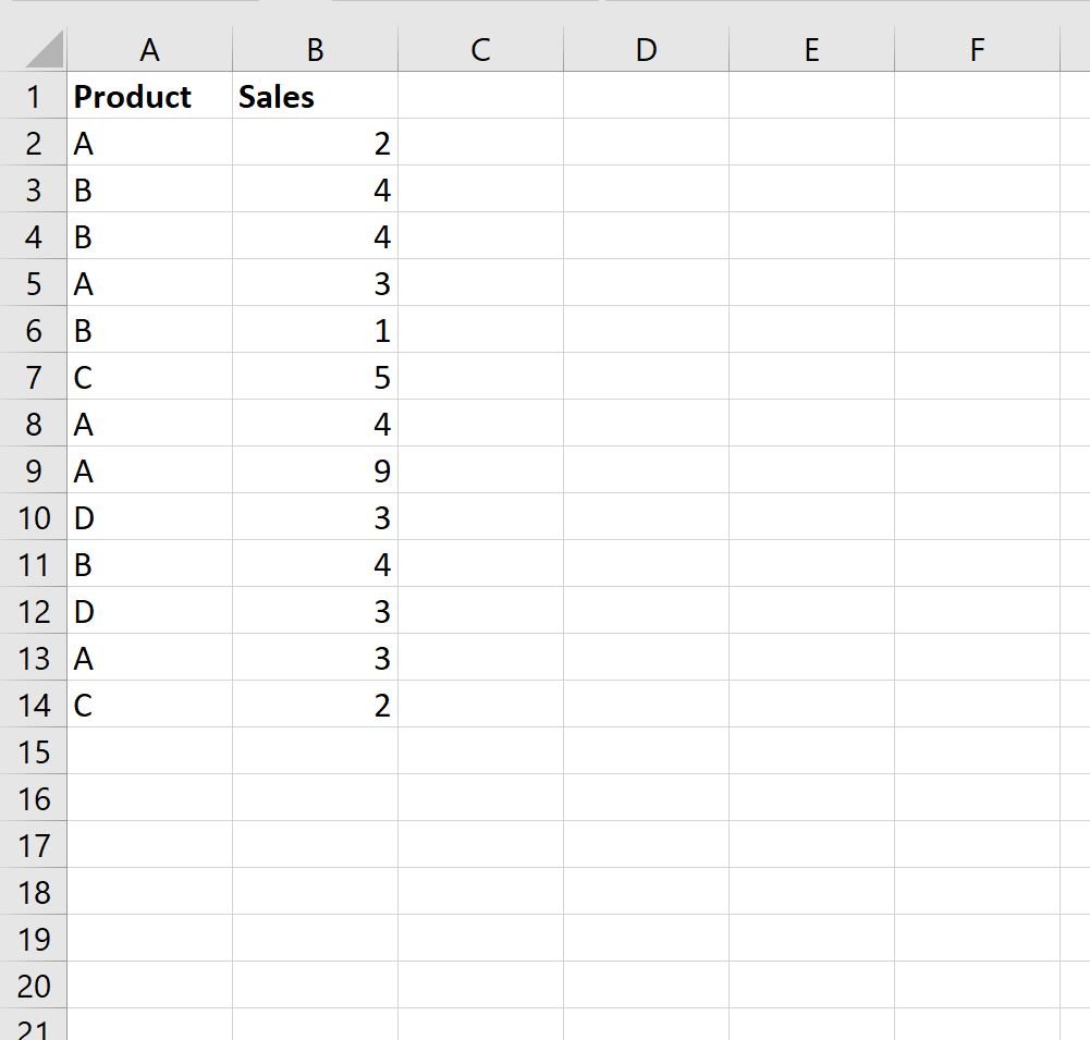
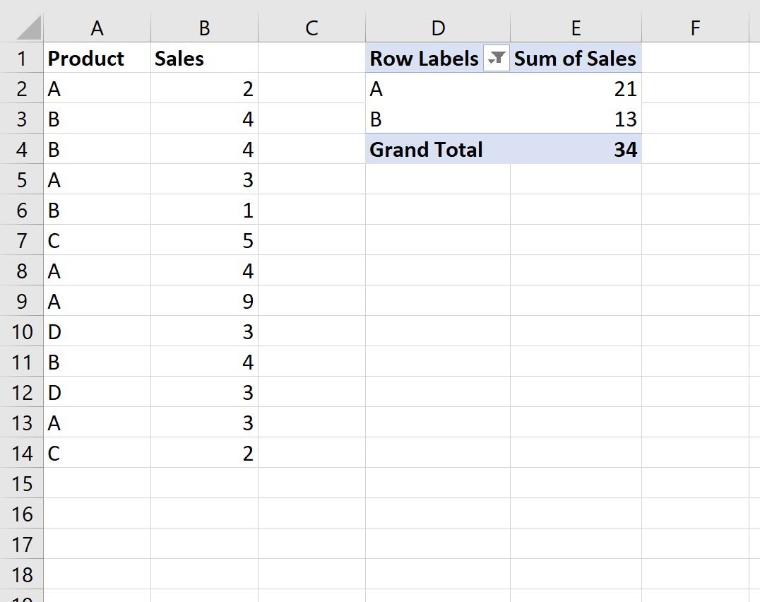
Suppose we have the following dataset in Excel that shows the number of sales of four different products:
Now suppose we create the following pivot table to summarize the total sales for each product:
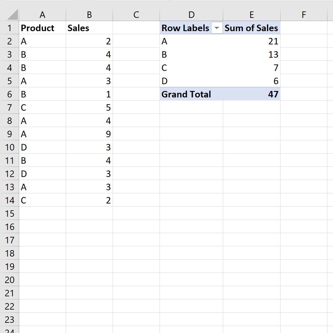
Now suppose we would like to filter the pivot table to only show rows where the Sum of Sales is greater than 10.
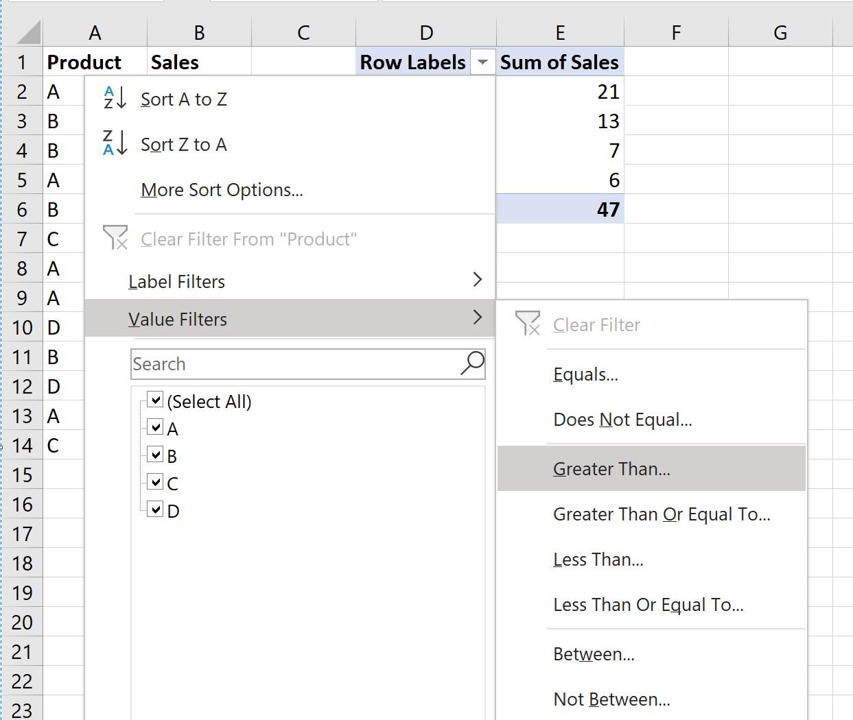
To do so, click the dropdown arrow next to Row Labels, then click Value Filters, then click Greater Than:
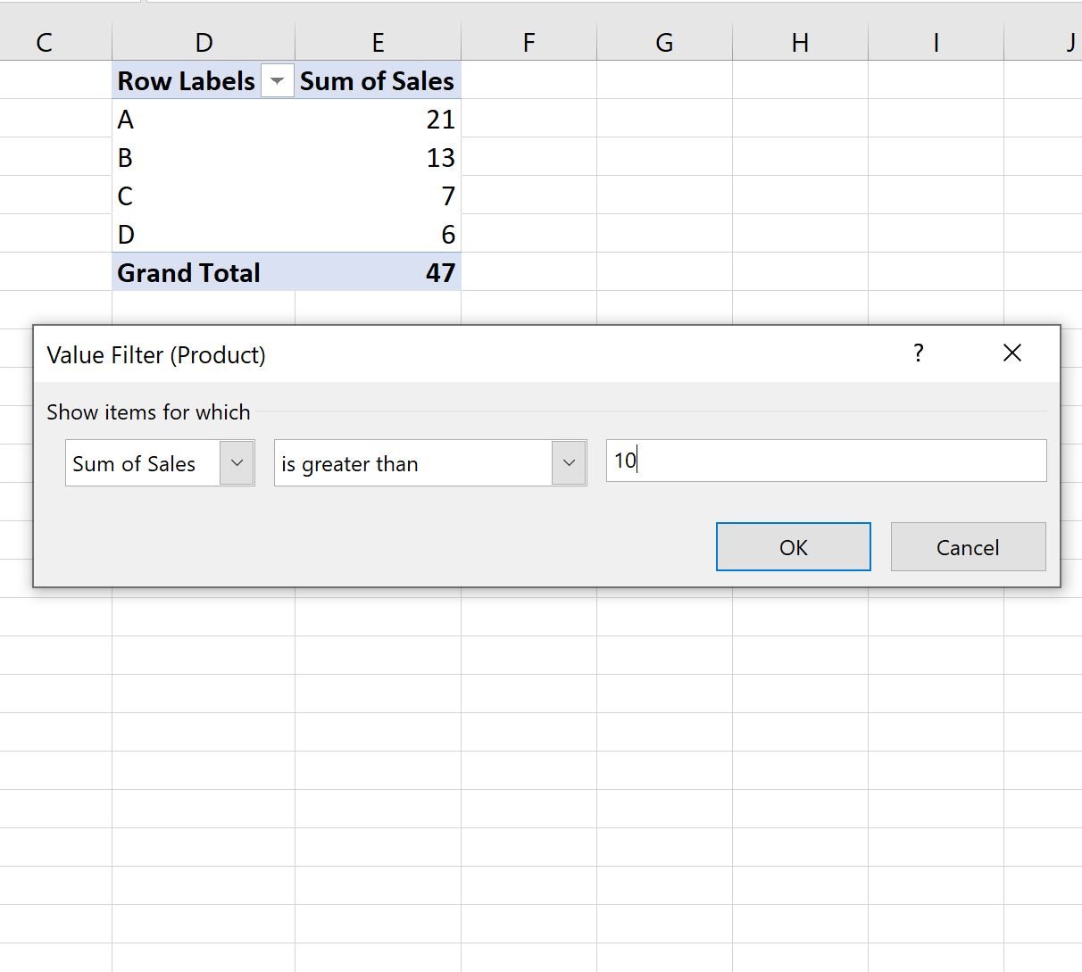
In the window that appears, type 10 in the blank space and then click OK:
The pivot table will automatically be filtered to only show rows where the Sum of Sales is greater than 10:
To remove the filter, simply click the dropdown arrow next to Row Labels again and then click Clear Filter From “Product.”
Additional Resources
The following tutorials explain how to perform other common operations in Excel:
Excel: How to Filter Top 10 Values in Pivot Table
Excel: How to Sort Pivot Table by Grand Total
Excel: How to Calculate the Difference Between Two Pivot Tables