Often you may want to filter the rows in a pivot table in Excel by a specific date range.
Fortunately this is easy to do using the Date Filters option in the dropdown menu within the Row Labels column of a pivot table.
The following example shows exactly how to do so.
Example: Filter Pivot Table by Date Range in Excel
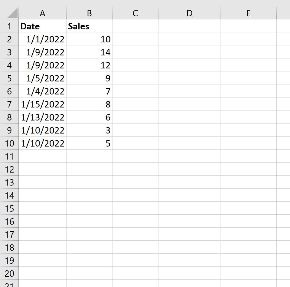
Suppose we have the following dataset in Excel that shows the number of sales on various dates:
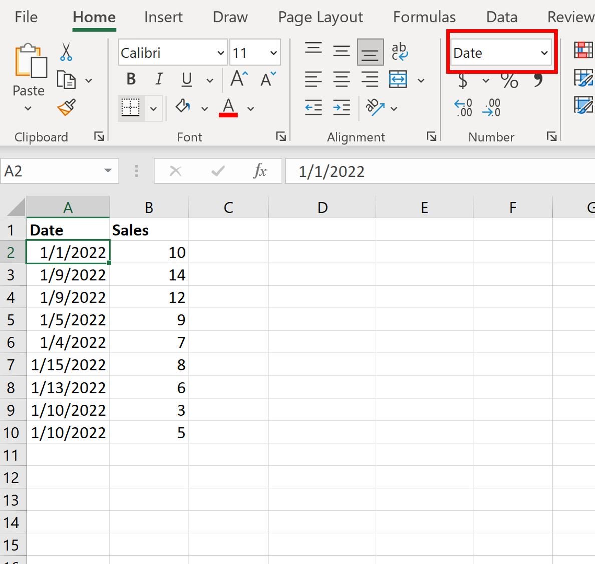
Before creating a pivot table for this data, click on one of the cells in the Date column and make sure that Excel recognizes the cell as a Date format:
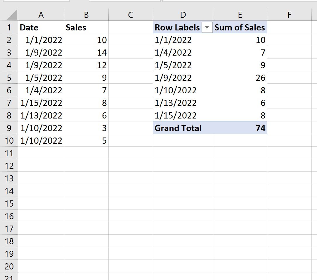
Next, we can highlight the cell range A1:B10, then click the Insert tab along the top ribbon, then click PivotTable, and insert the following pivot table to summarize the total sales for each date:
Now suppose we would like to filter the pivot table to only show the dates between 1/5/2022 and 1/13/2022.
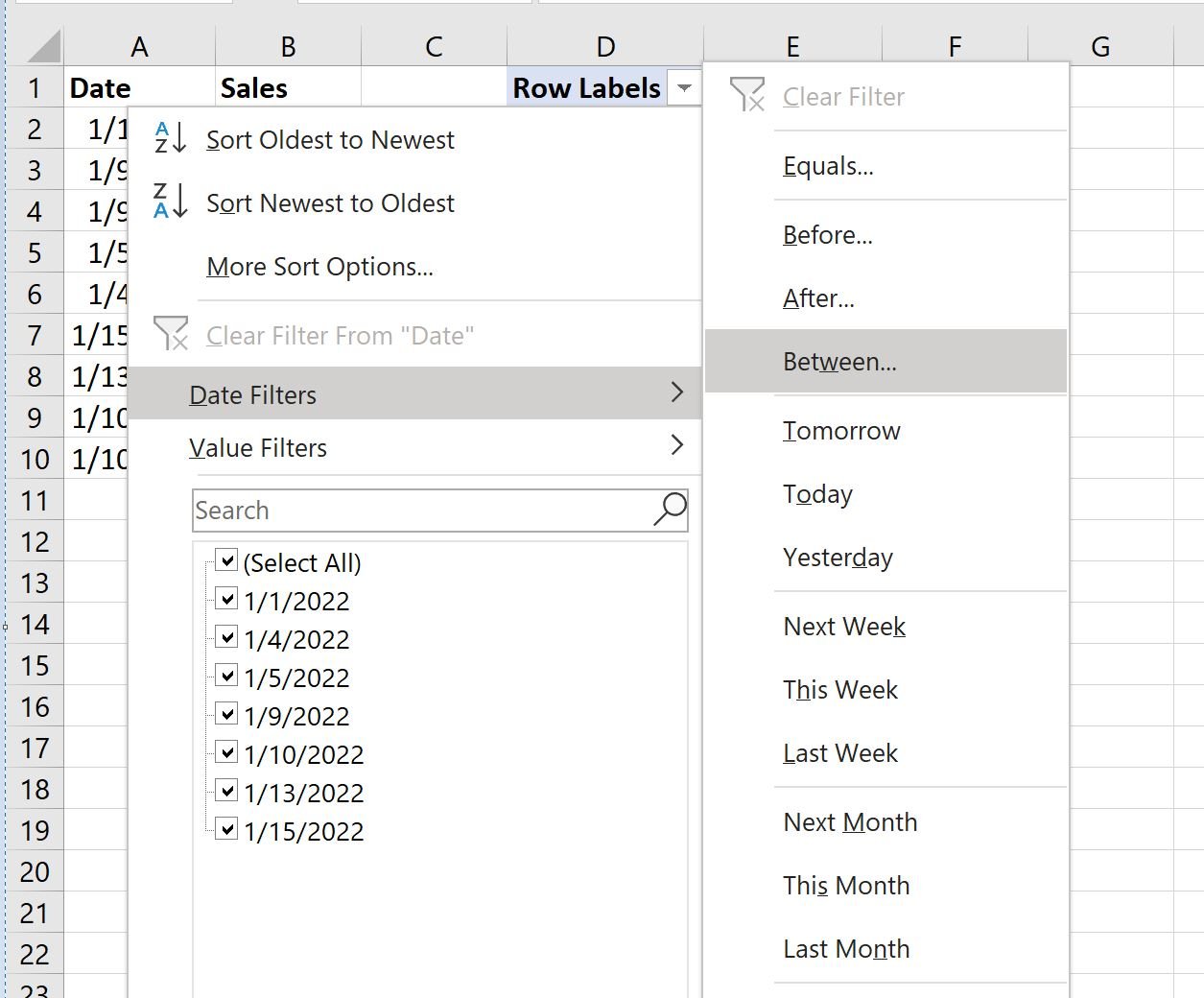
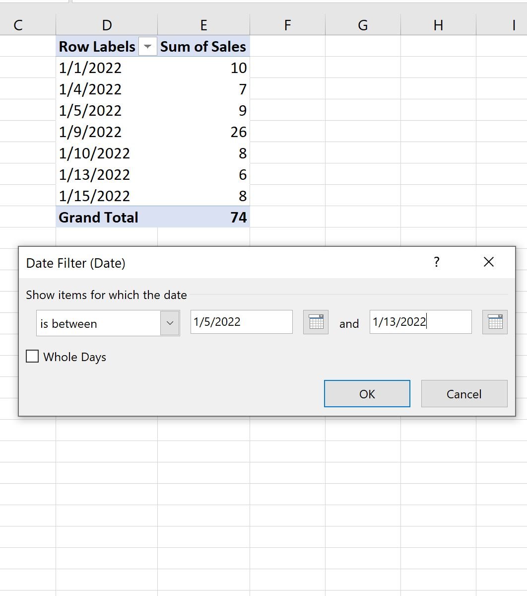
To apply this filter, click the dropdown arrow next to Row Labels, then click Date Filters, then click Between:
In the new window that appears, type 1/5/2022 and 1/13/2022 into the boxes for the date range:
Once you click OK, the rows in the pivot table will automatically be filtered to only show this date range:
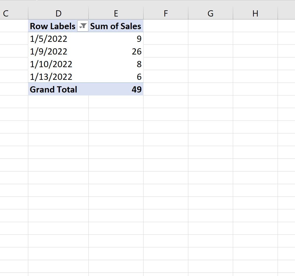
To remove this filter, simply click the filter icon next to Row Labels and then click Clear Filter from Date.
Additional Resources
The following tutorials explain how to perform other common operations in Excel:
Excel: How to Filter Top 10 Values in Pivot Table
Excel: How to Sort Pivot Table by Grand Total
Excel: How to Calculate the Difference Between Two Pivot Tables