The following step-by-step example shows how to delete a calculated field from a pivot table in Excel.
Step 1: Create the Pivot Table
Suppose we create the following pivot table that summarizes the total sales and returns at three different stores:

Step 2: Add Calculated Field to Pivot Table
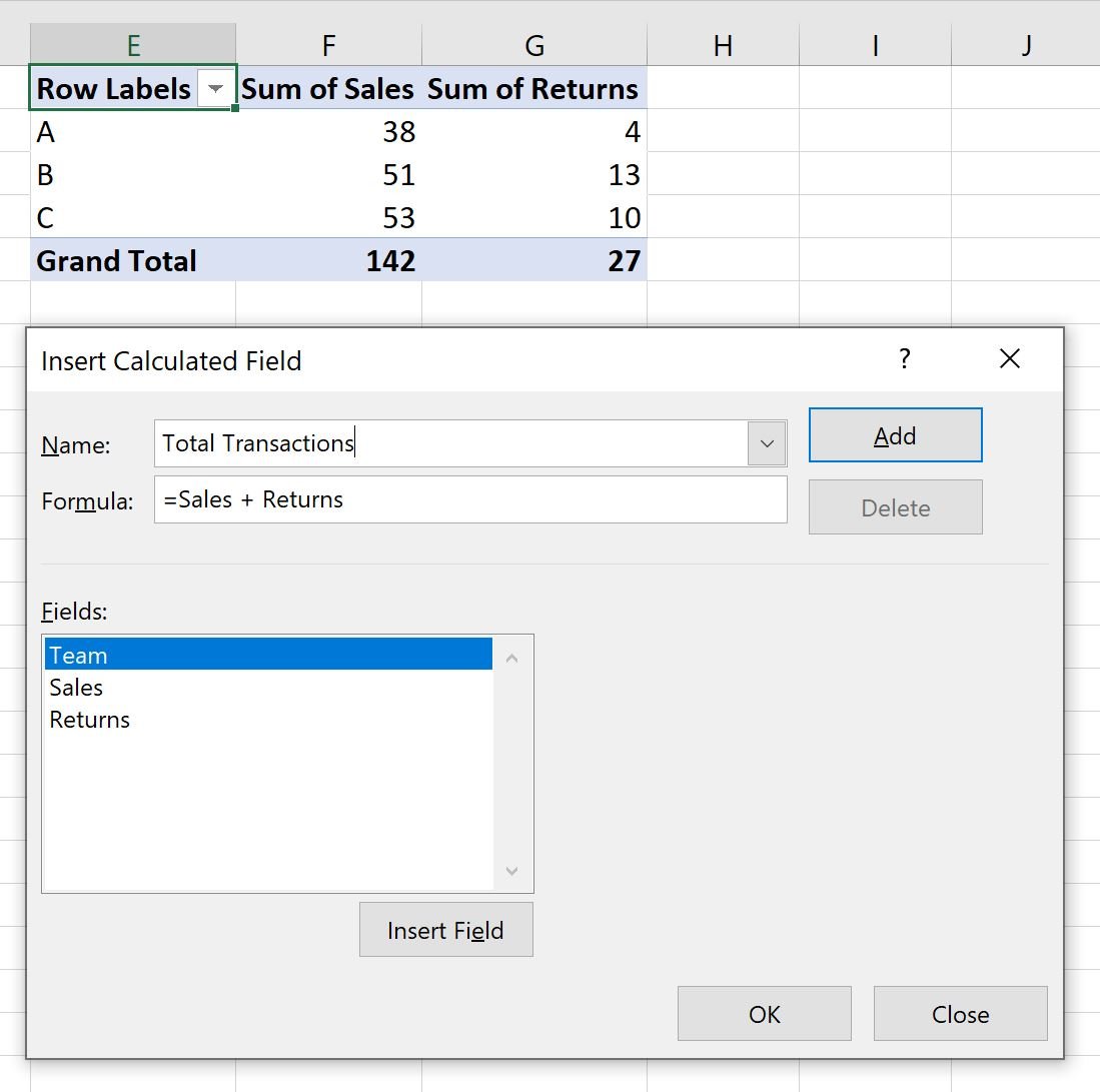
Suppose we would like to create a new column in the pivot table that displays the sum of the Sum of Sales and Sum of Returns columns.
To do so, we need to add a calculated field to the pivot table by clicking on any value in the pivot table, then clicking the PivotTable Analyze tab, then clicking Fields, Items & Sets, then Calculated Field:

In the new window that appears, type “Total Transactions” in the Name field, then type = Sales + Returns in the Formula field.
Then click Add, then click OK.

This calculated field will automatically be added to the pivot table:

Step 3: Delete Calculated Field from Pivot Table
Now suppose we would like to delete the calculated field from the pivot table.
To do so, we can click the Calculated Field insert button again:

In the window that appears, choose Total Transactions from the Name dropdown menu.
Then click the Delete button, then click OK:

The calculated field will be removed from the pivot table:

Additional Resources
The following tutorials explain how to perform other common tasks in Excel:
How to Sum Two Columns in a Pivot Table in Excel
How to Subtract Two Columns in a Pivot Table in Excel
Excel: Find Percentage Difference Between Two Columns in Pivot Table