Often you may want to create a chart in Excel using a range of data and ignore any blank cells in the range.
Fortunately this is easy to do using the Hidden and Empty Cells feature in Excel.
The following example shows how to use this function in practice.
Example: Create Chart in Excel and Ignore Blank Cells
Suppose we have the following dataset that shows the sales of some product during each month in a year:
![]()
Now suppose we would like to create a line chart to visualize the sales during each month.
We can highlight the cells in the range B2:B13, then click the Insert tab along the top ribbon, then click the Line button within the Charts group:
![]()
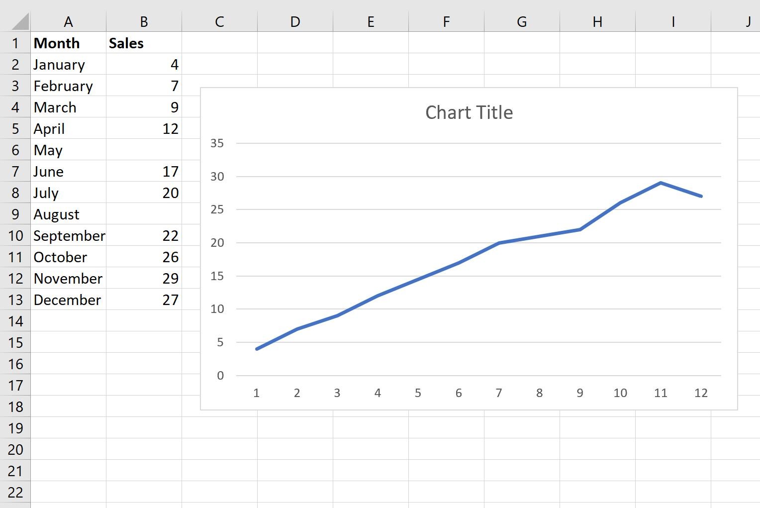
The following line chart will appear:
![]()
Notice that there are two gaps in the line chart where we have missing values for the months of May and August.
To fill in these gaps, right click anywhere on the chart and then click Select Data:
![]()
In the new window that appears, click the Hidden and Empty Cells button in the bottom left corner:
![]()
In the new window that appears, check the button next to Connect data points with line and then click OK:
![]()
The gaps in the line chart will automatically be filled in:
Additional Resources
The following tutorials explain how to perform other common tasks in Excel:
How to Replace #N/A Values in Excel
How to Interpolate Missing Values in Excel
How to Count Duplicates in Excel