Placing numeric data into bins is a useful way to summarize the distribution of values in a dataset.
The following example shows how to perform data binning in Excel.
Example: Data Binning in Excel
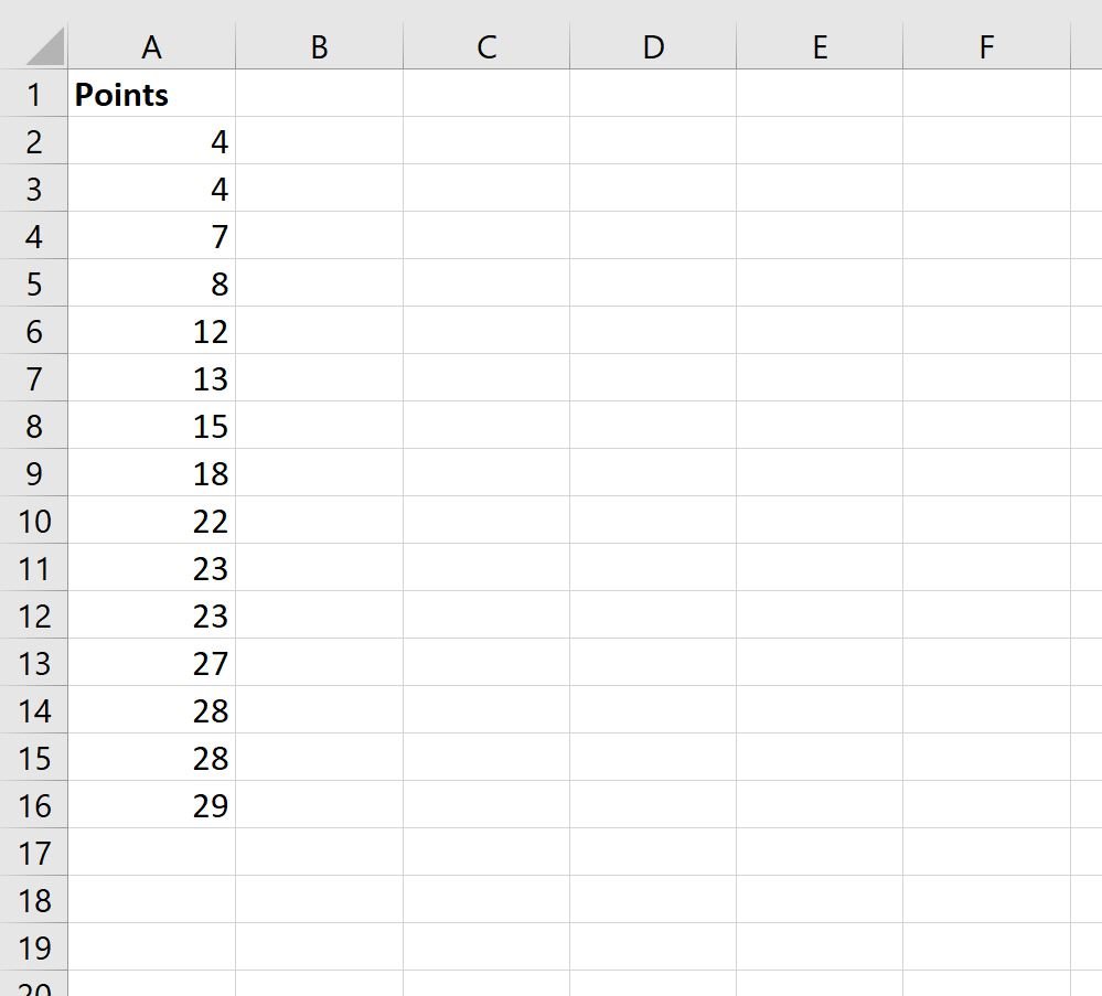
Suppose we have the following dataset that shows the number of points scored by various basketball players:
To place each of the values into bins, we can create a new column that defines the largest value for each bin:
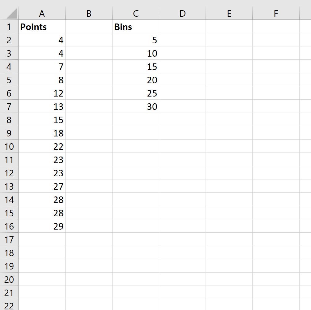
In this example, we have specified the following bins:
- 0-5
- 6-10
- 11-15
- 16-20
- 21-25
- 26-30
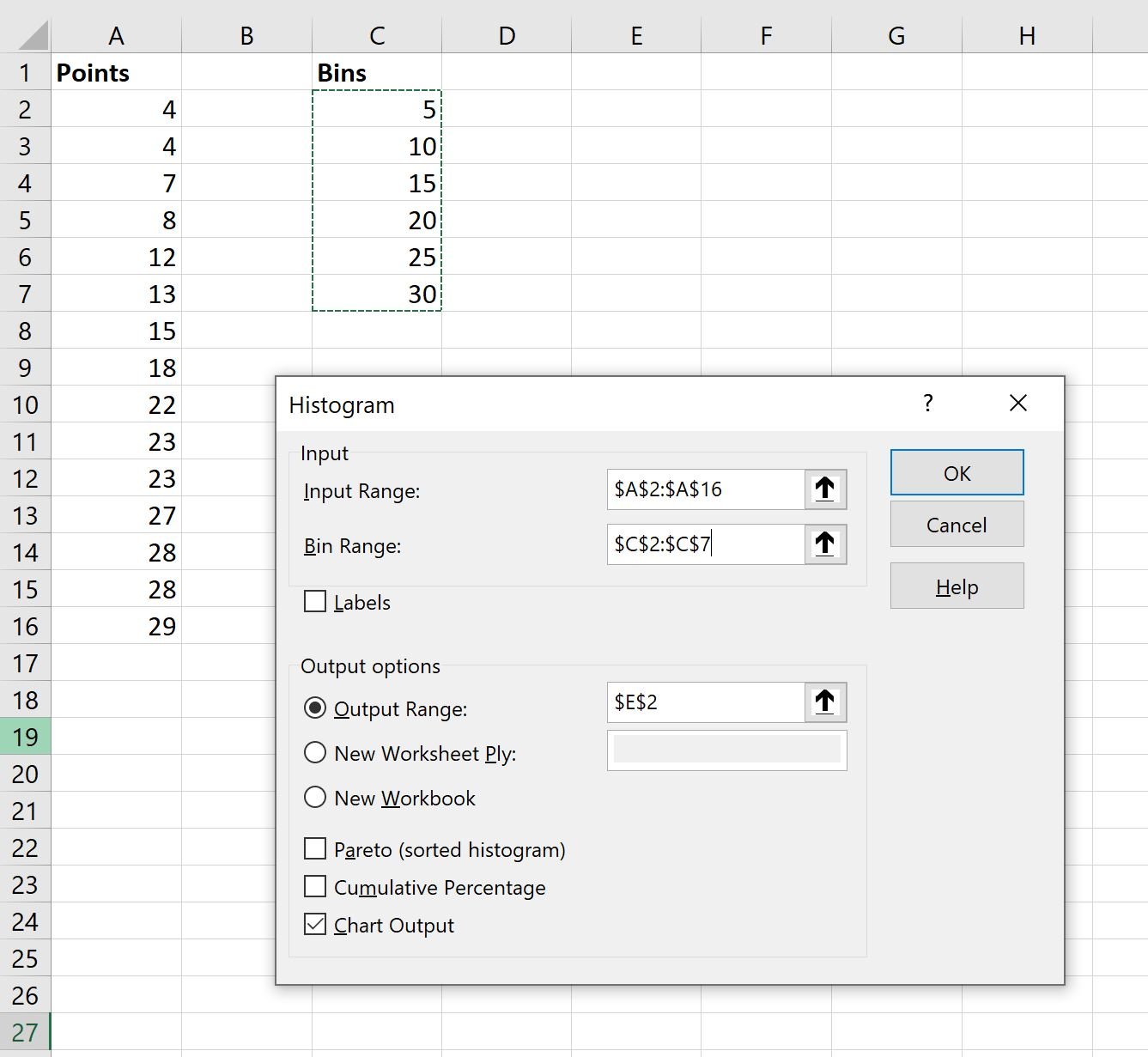
To calculate how many data values fall into each bin, click the Data tab along the top ribbon, then click Data Analysis within the Analyze group.
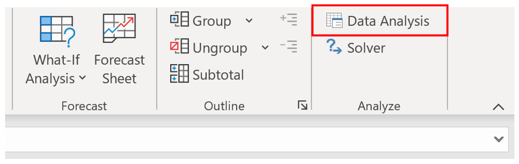
Note: If you don’t see an option for Data Analysis, you need to first load the free Analysis Toolpak in Excel.
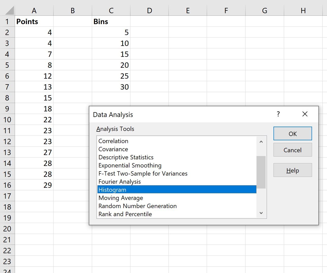
In the new window that appears, click Histogram, then click OK:
Choose A2:A16 as the Input Range, C2:C7 as the Bin Range, E2 as the Output Range, and check the box next to Chart Output. Then click OK.
The number of values that fall into each bin will automatically be calculated:
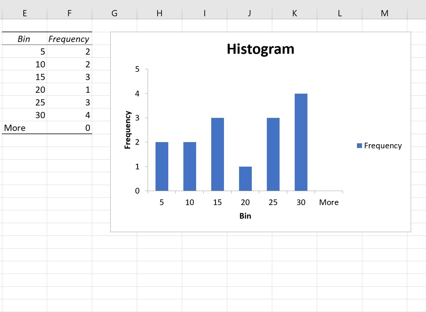
From the output we can see:
- 2 values fall into the 0-5 bin.
- 2 values fall into the 6-10 bin.
- 3 values fall into the 11-15 bin.
- 1 value falls into the 16-20 bin.
- 3 values fall into the 21-25 bin.
- 4 values fall into the 26-30 bin.
- 0 values are greater than 30.
The histogram allows us to visualize this distribution of data values as well.
Note: In this example, we chose to make each bin the same width but we can make individual bins different sizes if we’d like.
Additional Resources
The following tutorials explain how to perform other common operations in Excel:
Excel: How to Filter Top 10 Values in Pivot Table
Excel: How to Sort Pivot Table by Grand Total
Excel: How to Calculate the Difference Between Two Pivot Tables