In statistics, we’re often interested in understanding the relationship between two variables. For example, we might want to understand the relationship between the number of hours a student studies and the exam score they receive.
One way to quantify this relationship is to use the Pearson correlation coefficient, which is a measure of the linear association between two variables. It has a value between -1 and 1 where:
- -1 indicates a perfectly negative linear correlation between two variables
- 0 indicates no linear correlation between two variables
- 1 indicates a perfectly positive linear correlation between two variables
The further away the correlation coefficient is from zero, the stronger the relationship between the two variables.
But in some cases we want to understand the correlation between more than just one pair of variables. In these cases, we can create a correlation matrix, which is a square table that shows the the correlation coefficients between several pairwise combination of variables.
In this tutorial we explain how to create a correlation matrix in Stata.
How to Create a Correlation Matrix in Stata
The command corr can be used to produce a correlation matrix for a particular dataset in Stata.
To illustrate this, let’s load the 1980 census data into Stata by typing the following into the command box:
use http://www.stata-press.com/data/r13/census13
We can then get a quick summary of the dataset by typing the following into the command box:
summarize
This produces the following table:
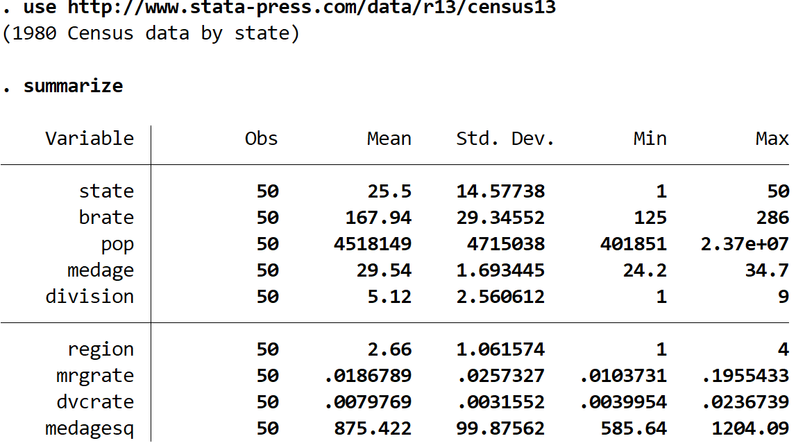
We see that the dataset contains nine different variables. To create a correlation matrix for every pairwise combination of variables in the dataset, we can type the following into the command box:
corr
This produces the following correlation matrix:
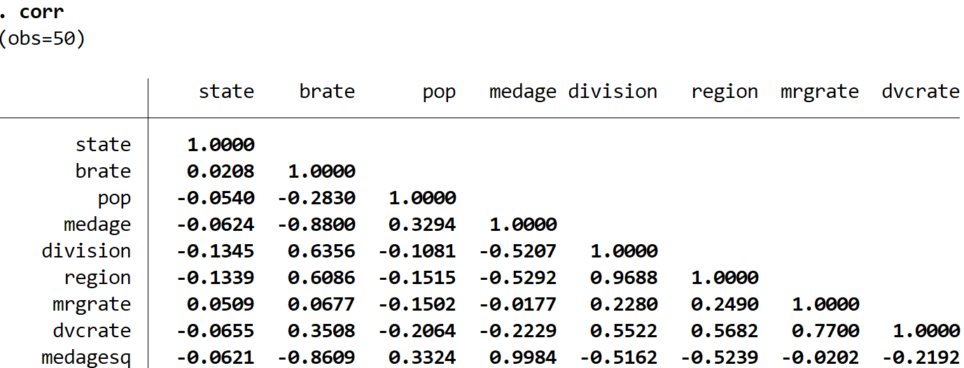
The numbers shown in the table represent the Pearson Correlation Coefficients for each pairwise combination of variables. For example, the correlation between pop and state is -0.0540. This indicates that these two variables are slightly negatively correlated.
Notice that the correlation along the diagonals of the table are each 1.0000, since each variable is perfectly correlated with itself.
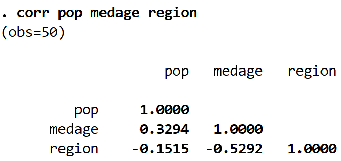
You can also create a correlation matrix for only a certain subset of variables in a dataset by specifying the variables after the corr command. For example, here is how to create a correlation matrix for just the variables pop, medage, and region:
corr pop medage region
This produces the following correlation matrix for just these three variables:
It’s also possible to put a star next to the correlation coefficients that are statistically significant at a certain significance level by using the pwcorr command (which produces the same result as corr) along with the star() command.
For example, the following code produces a correlation matrix for every variable in the census dataset and places a star next to the correlation coefficients that are statistically significant at α = 0.05:
pwcorr, star(.05)
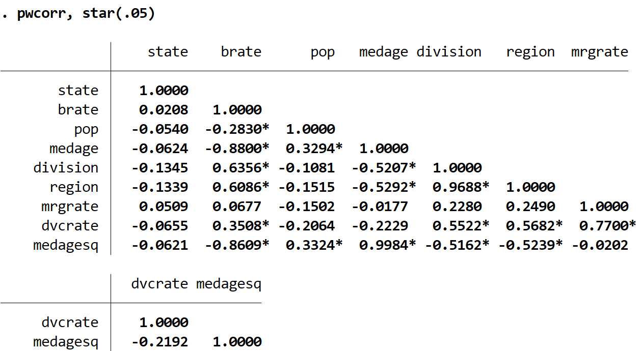
Notice how several of the correlation coefficients in the table are statistically significant at α = 0.05. We could set α to be any number we’d like, but common choices are .01, .05, and .10.
In general, the lower we set the value of α, the fewer correlation coefficients will be statistically significant. For example, suppose we set α = 0.01.
pwcorr, star(.01)
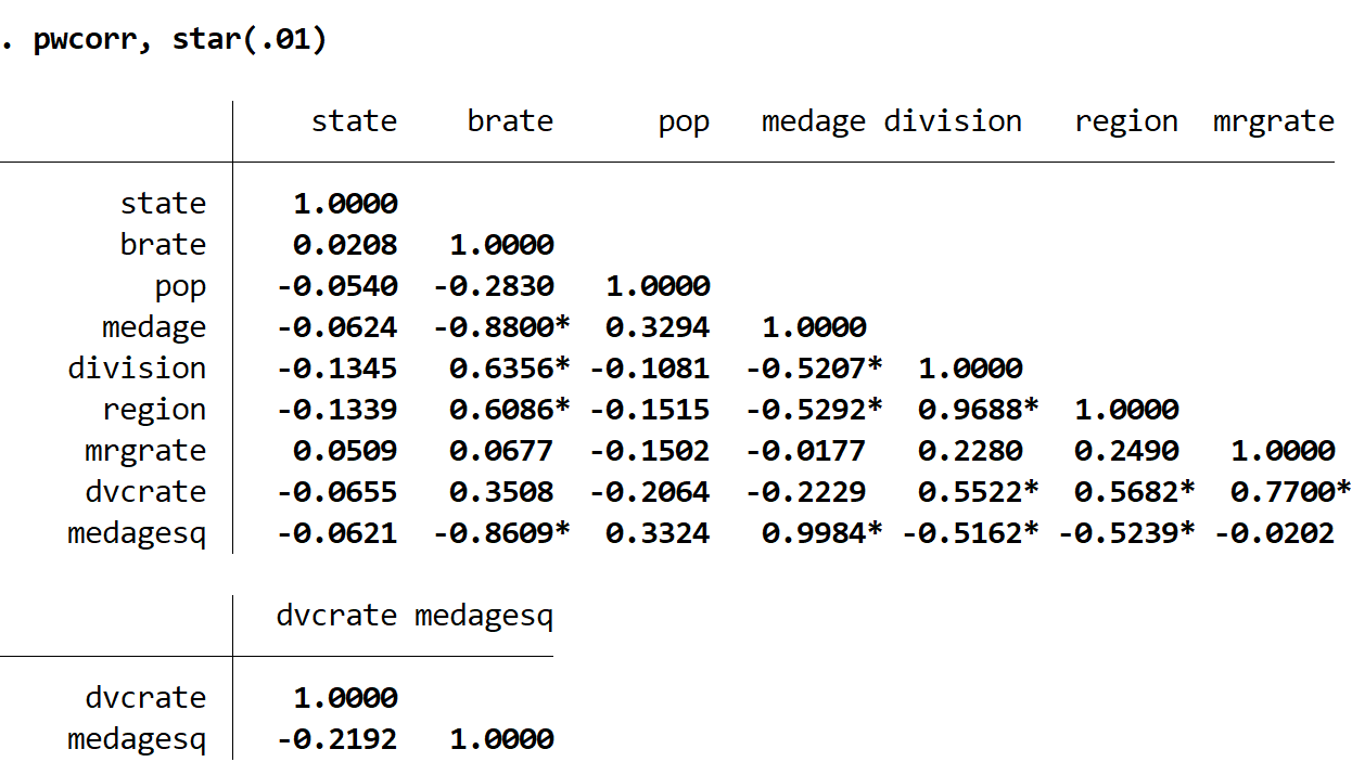
Notice how fewer correlation coefficients have a star next to them.