The central limit theorem states that the sampling distribution of a sample mean is approximately normal if the sample size is large enough, even if the population distribution is not normal.
The central limit theorem also states that the sampling distribution will have the following properties:
1. The mean of the sampling distribution will be equal to the mean of the population distribution:
x = μ
2. The standard deviation of the sampling distribution will be equal to the standard deviation of the population distribution divided by the sample size:
s = σ / n
The following example demonstrates how to apply the central limit theorem in R.
Example: Applying the Central Limit Theorem in R
Suppose the width of a turtle’s shell follows a uniform distribution with a minimum width of 2 inches and a maximum width of 6 inches.
That is, if we randomly selected a turtle and measured the width of its shell, it’s equally likely to be any width between 2 and 6 inches.
The following code shows how to create a dataset in R that contains the measurements of shell widths for 1,000 turtles, uniformally distributed between 2 and 6 inches:
#make this example reproducible
set.seed(0)

#create random variable with sample size of 1000 that is uniformally distributed
data #create histogram to visualize distribution of turtle shell widths
hist(data, col='steelblue', main='Histogram of Turtle Shell Widths')

Notice that the distribution of turtle shell widths is not normally distributed at all.
Now, imagine that we take repeated random samples of 5 turtles from this population and measure the sample mean over and over again.
The following code shows how to perform this process in R and create a histogram to visualize the distribution of sample means:
#create empty vector to hold sample means
sample5 #take 1,000 random samples of size n=5
n = 1000
for (i in 1:n){
sample5[i] = mean(sample(data, 5, replace=TRUE))
}

#calculate mean and standard deviation of sample means
mean(sample5)

[1] 4.008103

sd(sample5)

[1] 0.5171083

#create histogram to visualize sampling distribution of sample means
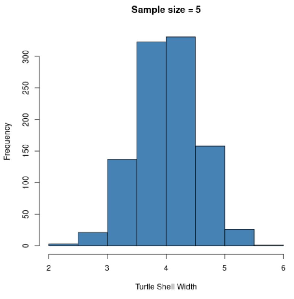
hist(sample5, col ='steelblue', xlab='Turtle Shell Width', main='Sample size = 5')

Notice that the sampling distribution of sample means appears normally distributed, even though the distribution that the samples came from was not normally distributed.
Also notice the sample mean and sample standard deviation for this sampling distribution:
- x̄: 4.008
- s: 0.517
Now suppose we increase the sample size that we use from n=5 to n=30 and recreate the histogram of sample means:
#create empty vector to hold sample means
sample30 #take 1,000 random samples of size n=30
n = 1000
for (i in 1:n){
sample30[i] = mean(sample(data, 30, replace=TRUE))
}

#calculate mean and standard deviation of sample means
mean(sample30)

[1] 4.000472

sd(sample30)

[1] 0.2003791

#create histogram to visualize sampling distribution of sample means
hist(sample30, col ='steelblue', xlab='Turtle Shell Width', main='Sample size = 30')

The sampling distribution is normally distributed once again, but the sample standard deviation is even smaller:
- s: 0.200
This is because we used a larger sample size (n = 30) compared to the previous example (n = 5) so the standard deviation of sample means is even smaller.
If we keep using larger and larger sample sizes, we’ll find that the sample standard deviation gets smaller and smaller.
This illustrates the central limit theorem in practice.
Additional Resources
The following resources provide additional information about the central limit theorem:
An Introduction to the Central Limit Theorem
Central Limit Theorem Calculator
5 Examples of Using the Central Limit Theorem in Real Life