How to Simulate & Plot a Bivariate Normal Distribution in R

In statistics, two variables follow a bivariate normal distribution if they have a normal distribution when added together.

This tutorial explains how to perform the following tasks in R:

• Simulate a bivariate normal distribution
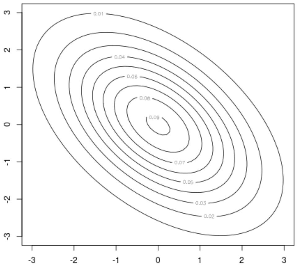
• Plot a bivariate normal distribution using a contour plot (2-D plot)
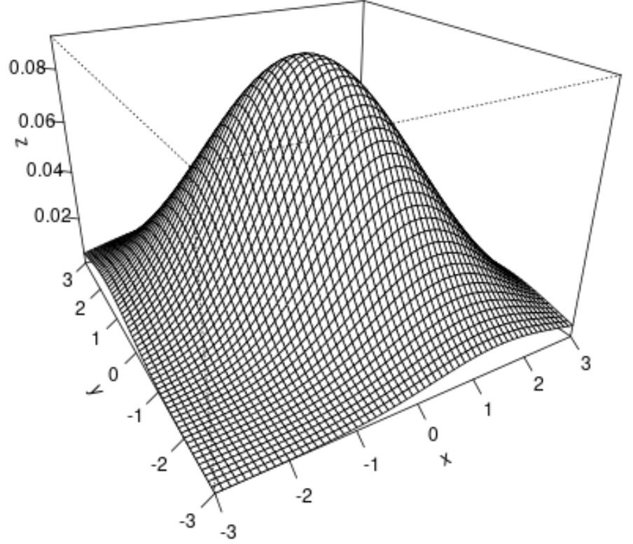
• Plot a bivariate normal distribution using a surface plot (3-D plot)

Let’s jump in!

Example 1: Simulate a Bivariate Normal Distribution in R

The easiest way to simulate a bivariate normal distribution in R is to use the mvrnorm() function from the MASS package.

The following code shows how to use this function to simulate a bivariate normal distribution in practice:

library(MASS)

#make this example reproducible
set.seed(0)

#simulate bivariate normal distribution
bivariate_data data.frame(mvrnorm(n=100,
                                        mu=c(0, 0),
                                        Sigma=matrix(c(5, 3, 4, 4), ncol=2)))

#view first six rows of bivariate dataset
head(bivariate_data)

           V1         V2
1 -2.03600343 -2.9623059
2  0.07719131  1.2948982
3 -3.26729701 -1.7928069
4 -2.62985132 -2.3015471
5 -1.75126215  0.3056698
6  3.67698436  2.2020238

Here’s what each argument in the mvrnorm() function does:

• n: Defines the sample size
• mu: Defines the mean of each variable
• Sigma: Defines the covariance matrix of the two variables

The end result is a data frame with two variables that follow a normal distribution when added together.

Example 2: Plot a Bivariate Normal Distribution

The easiest way to plot a bivariate normal distribution in R is to use functions from the mnormt() package.

For example, we can use the contour() function from this package to create a contour plot, which offers a 2-D visualization of the bivariate normal distribution:

library(mnormt)

#make this example reproducible
set.seed(0)

#create bivariate normal distribution
x     2)
f     #create contour plot
contour(x, y, z)

We can also use the persp() function from to create a surface plot, which offers a 3-D visualization of the bivariate normal distribution:

library(mnormt)

#make this example reproducible
set.seed(0)

#create bivariate normal distribution
x     2)
f     #create surface plot
persp(x, y, z, theta=-30, phi=25, expand=0.6, ticktype='detailed')

Here’s what each argument in the persp() function does:

• theta, phi: Defines the angles of the viewing direction.
• expand: Controls the size of the z-axis.
• ticktype: Controls the appearance of the ticks on the axes.

The end result is a 3-D surface plot of the bivariate normal distribution.

Additional Resources

The following tutorials explain how to work with other probability distributions in R:

How to Use the Normal Distribution in R
How to Use the Binomial Distribution in R
How to Use the Poisson Distribution in R
How to Use the Multinomial Distribution in R