Often you may want to group data by month in Google Sheets.
Fortunately this is easy to do using the pivot date group function within a pivot table.
The following step-by-step example shows how to use this function to group data by month in Google Sheets.
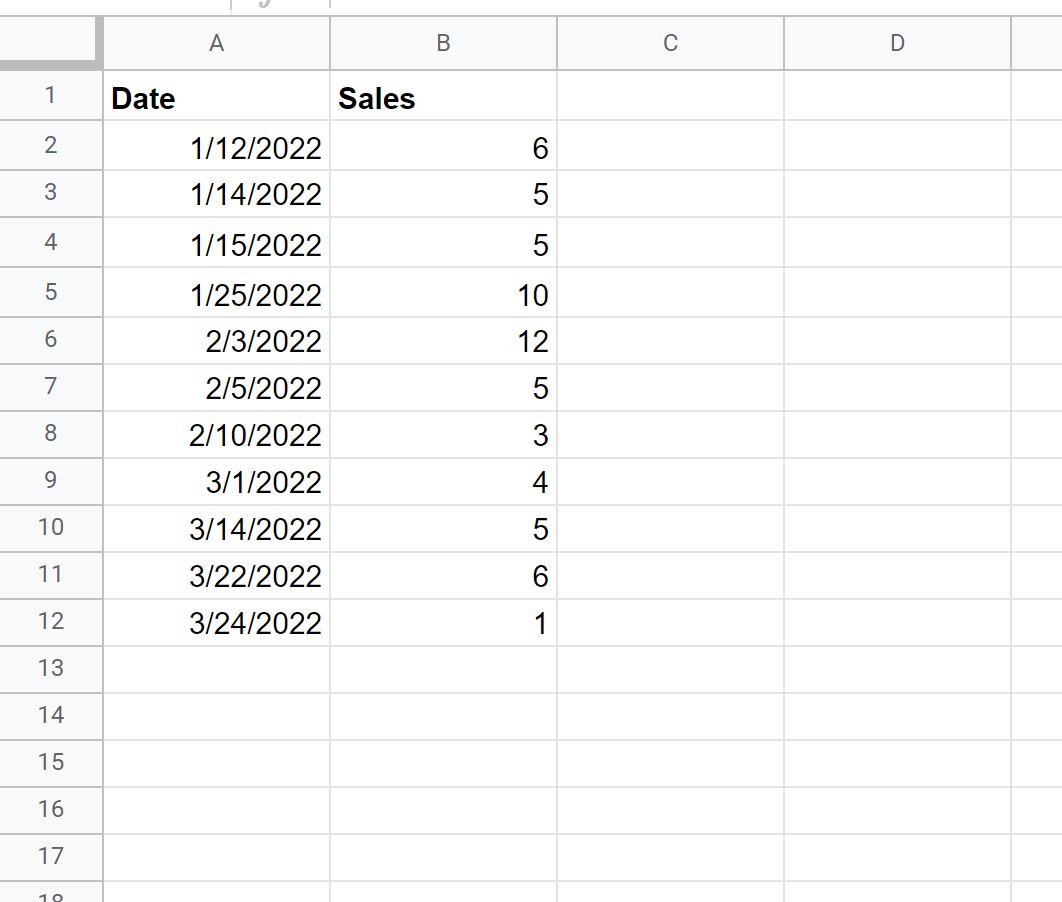
Step 1: Create the Data
First, let’s create a dataset that shows the total sales made by some company on various days:
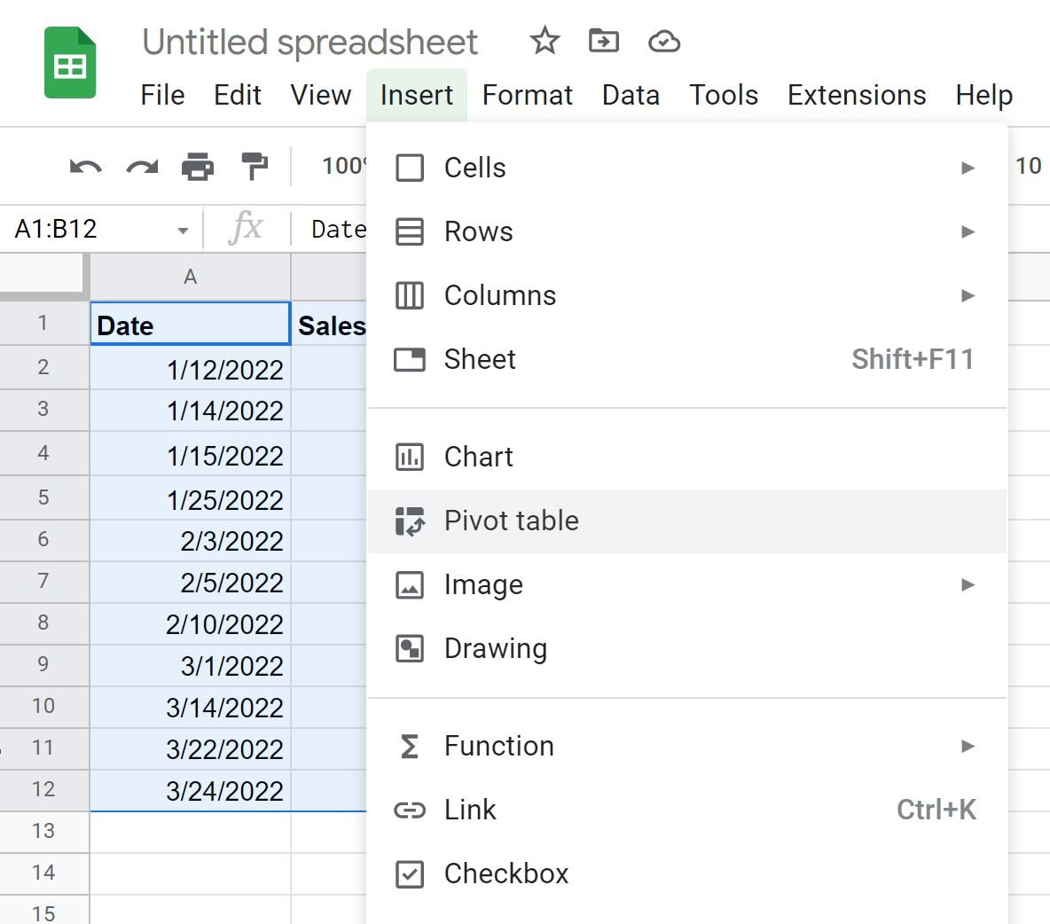
Step 2: Create a Pivot Table
Next, highlight the cells in the range A1:B12 and then click the Insert tab along the top ribbon and click Pivot table.
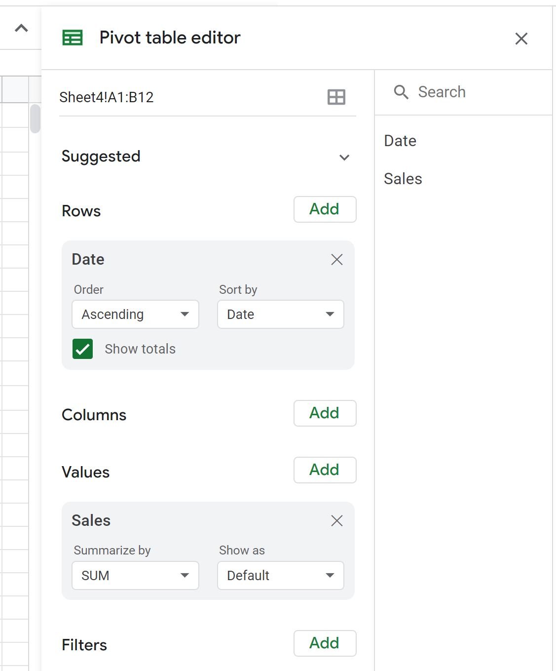
Next, we’ll choose to insert the pivot table in the current worksheet in cell D1:

In the Pivot table editor on the right side of the screen, choose Date for the Rows and Sales for the Values:
The values in the pivot table will now be filled in.
Step 3: Group the Data by Month
To group the data by month, right click on any value in the Date column of the pivot table and click Create pivot date group, then click Month:
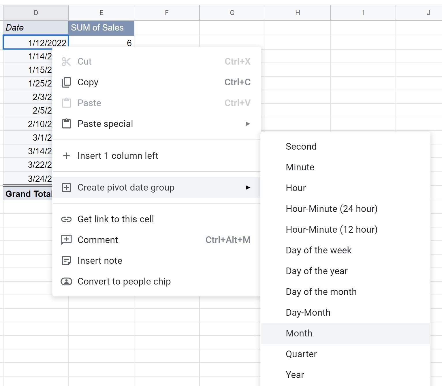
The data in the pivot table will automatically be grouped by month:
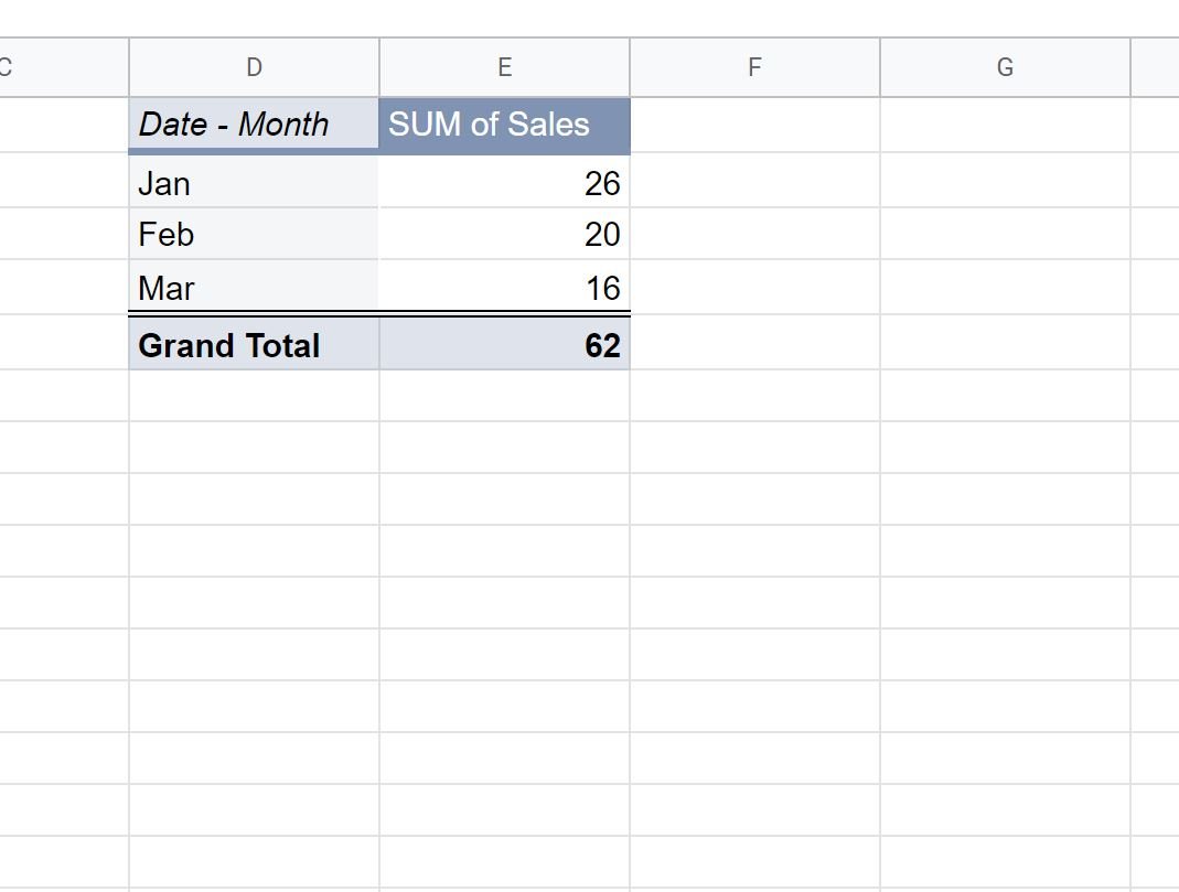
The pivot table now shows the sum of the sales grouped by month.
Additional Resources
The following tutorials explain how to perform other common operations in Google Sheets:
Google Sheets: How to Filter for Cells that Contain Text
Google Sheets: How to Use SUMIF with Multiple Columns
Google Sheets: How to Sum Across Multiple Sheets