Often you may want to calculate the median value in an Excel pivot table.
Unfortunately Excel doesn’t have a built-in feature to calculate the median, but you can use a MEDIAN IF function as a workaround.
The following step-by-step example shows how to do so.
Step 1: Enter the Data
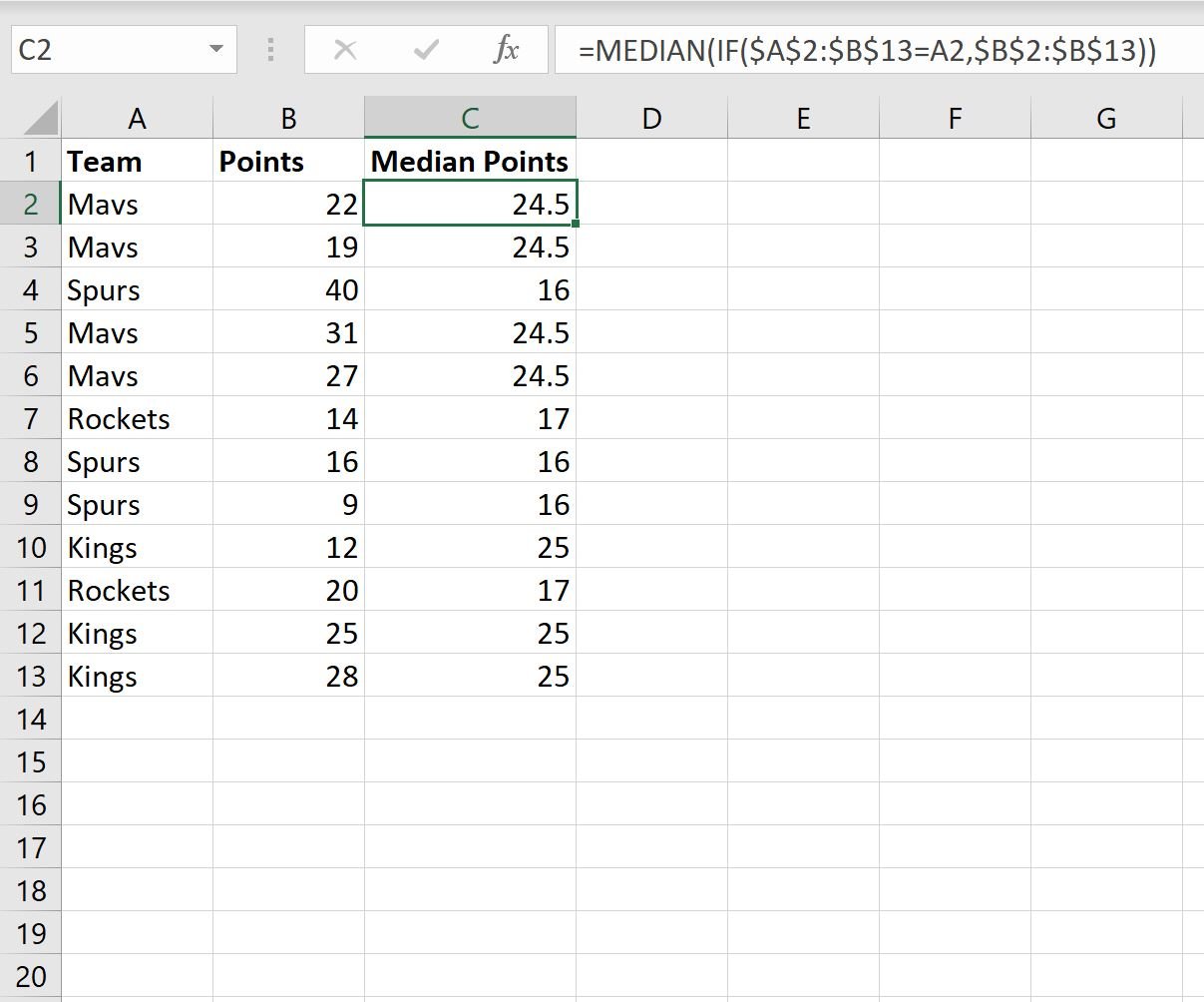
First, let’s enter the following data that shows the points scored by basketball players on various teams:

Step 2: Calculate the Median Value by Group
Next, we can use the following formula to calculate the median points value for each team:
=MEDIAN(IF($A$2:$B$13=A2,$B$2:$B$13))
The following screenshot shows how to use this formula in practice:
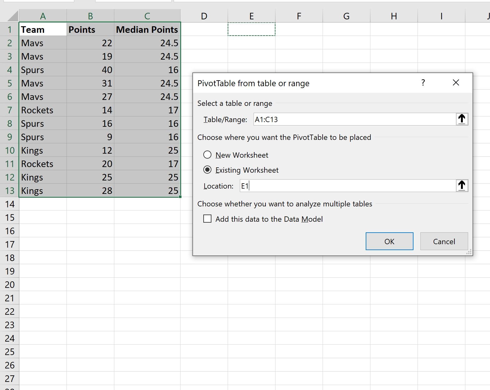
Step 3: Create the Pivot Table
To create a pivot table, click the Insert tab along the top ribbon and then click the PivotTable icon:

In the new window that appears, choose A1:C13 as the range and choose to place the pivot table in cell E1 of the existing worksheet:
Once you click OK, a new PivotTable Fields panel will appear on the right side of the screen.
Drag the Team field to the Rows box, then drag the Points and Median Points fields to the Values box:

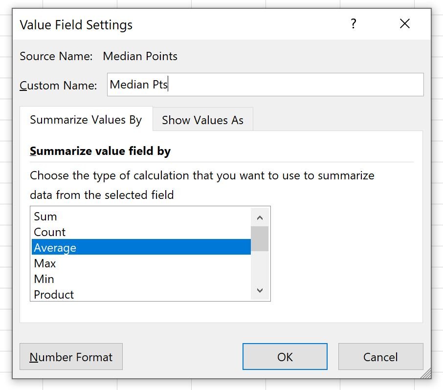
Next, click the Sum of Median Points dropdown arrow and then click Value Field Settings:

In the new window that appears, change the Custom Name to Median Pts and then click Average as the summarize value:
Once you click OK, the median points value for each team will be added to the pivot table:
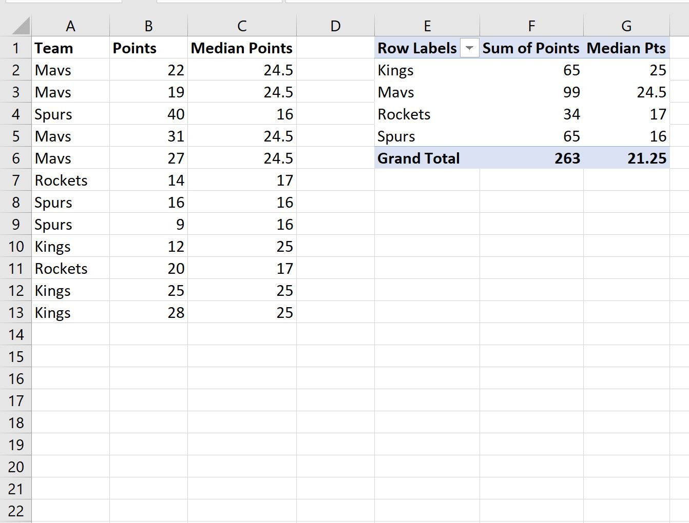
The pivot table now contains the following information:
- Each unique team name
- The sum of points scored by each team
- The median points scored by each team
Additional Resources
The following tutorials explain how to perform other common tasks in Excel:
How to Sort Pivot Table by Grand Total in Excel
How to Group Values in Pivot Table by Range in Excel
How to Group by Month and Year in Pivot Table in Excel