Often you may have one or more missing values in a series in Google Sheets that you’d like to fill in.
The following step-by-step example shows how to interpolate missing values in practice.
Step 1: Create the Data
First, let’s create a dataset in Google Sheets that contains some missing values:

Step 2: Calculate the Step Value
Next, we will use the following formula to determine what step value to use to fill in the missing data:
Step = (End – Start) / (#Missing observations + 1)
For this example, we would calculate the step value as:
Step = (35 – 20) / (4 – 1) = 3
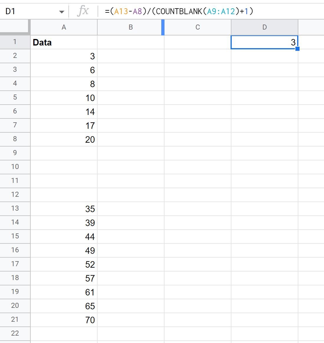
We can type the following formula into cell D1 to automatically calculate this value:
=(A13-A8)/(COUNTBLANK(A9:A12)+1)
The following screenshot shows how to use this formula in practice:
Step 3: Interpolate the Missing Values
Next, we need to add the step value to the missing values, starting with the first missing value:
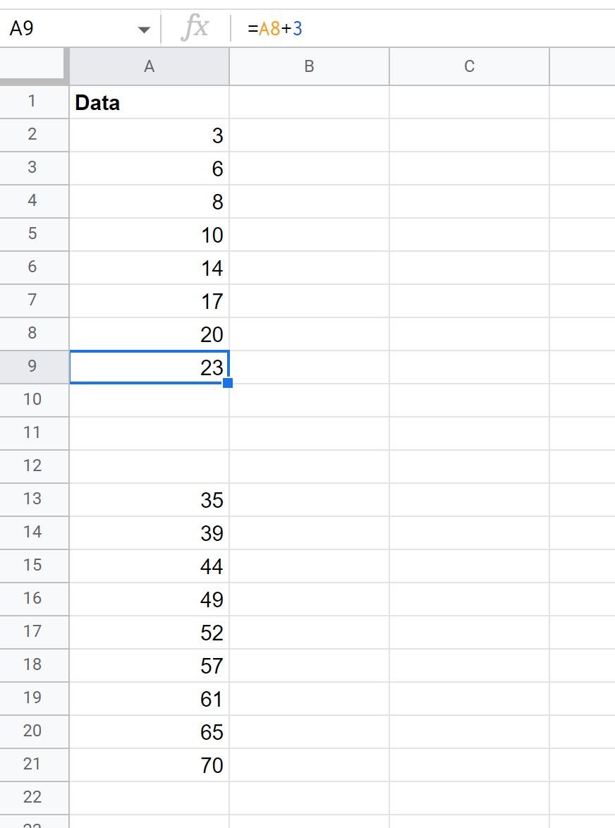
We can then drag and fill this formula down to each remaining blank cell:

Step 4: Visualize the Interpolated Values
Lastly, we can create a line chart to see if the interpolated values seem to fit the dataset well.
To do so, highlight cells A2:A21, then click the Insert tab, then click Chart.
In the Chart editor panel that appears on the right side of the screen, choose Line chart as the Chart type.
The following line chart will appear:

The interpolated values seem to fit the trend of the dataset well.
Additional Resource
The following tutorials explain how to perform other common tasks in Google Sheets:
How to Add Multiple Trendlines to Chart in Google Sheets
How to Add a Vertical Line to a Chart in Google Sheets
How to Add Average Line to Chart in Google Sheets