To apply conditional formatting to cells in Excel based on date values, you can use the New Rule option under the Conditional Formatting dropdown menu within the Home tab.

You can then choose the option called Use a formula to determine which cells to format and type a custom formula in the box:

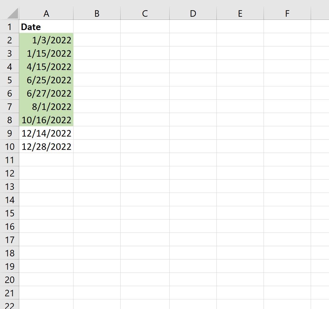
The following examples show how to use various formulas to highlight cells in the range A2:A10 in Excel that contain the following date values:

Example 1: Highlight Cells Based on Their Date Compared to Today
This article was written on 11/2/2022. Thus, we can use the following formula to highlight all cells in the range A2:A10 that have a date before today:

Once we press OK, all cells that have a date before 11/2/2022 will be highlighted:

Note that you can use the following formulas to highlight cells that are equal to or greater than today:
- Highlight cells with a date equal to today: =$A2 = TODAY()
- Highlight cells with a date after today: =$A2 > TODAY()
Example 2: Highlight Cells Based on Their Date Compared to Specific Date
We can use the following formula to highlight all cells in the range A2:A10 that have a date before 6/30/2022:

Once we press OK, all cells that have a date before 6/30/2022 will be highlighted:

Note: If your specific date is stored in a cell, such as cell D2, then you can instead use the following formula: =$A2 .
Example 3: Highlight Cells Based on Date Range
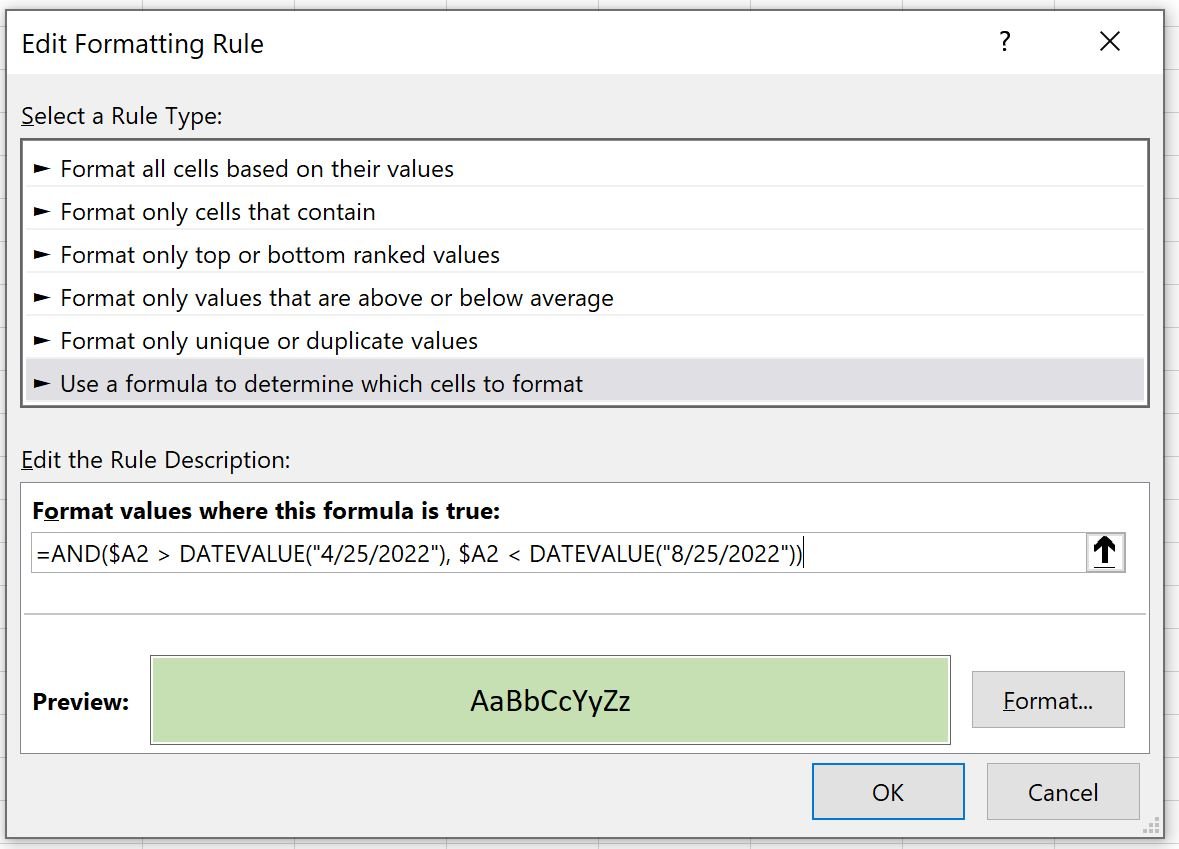
We can use the following formula to highlight all cells in the range A2:A10 that have a date between 4/25/2022 and 8/25/2022:

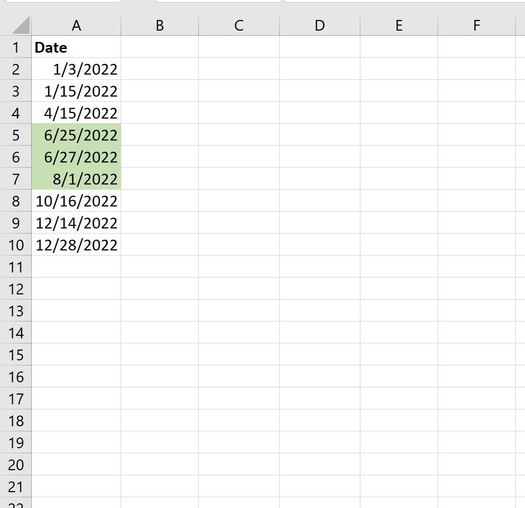
Once we press OK, all cells that have a date between this date range will be highlighted:

Notice that only the cells with a date between 4/25/2022 and 8/25/2022 are highlighted.
Additional Resources
The following tutorials explain how to perform other common tasks in Excel:
Excel: Apply Conditional Formatting if Cell Contains Text
Excel: Apply Conditional Formatting with Multiple Conditions
Excel: Apply Conditional Formatting if Between Two Values