You can use the following basic syntax to query from multiple ranges in Google Sheets:
=QUERY({Sheet1!A1:B10; Sheet2!A2:B5})
This particular example will return the cells in the range A1:B10 from Sheet1 stacked on top of the cells in the range A2:B5 from Sheet2.
The following example shows how to use this syntax in practice.
Example: Query From Multiple Ranges in Google Sheets
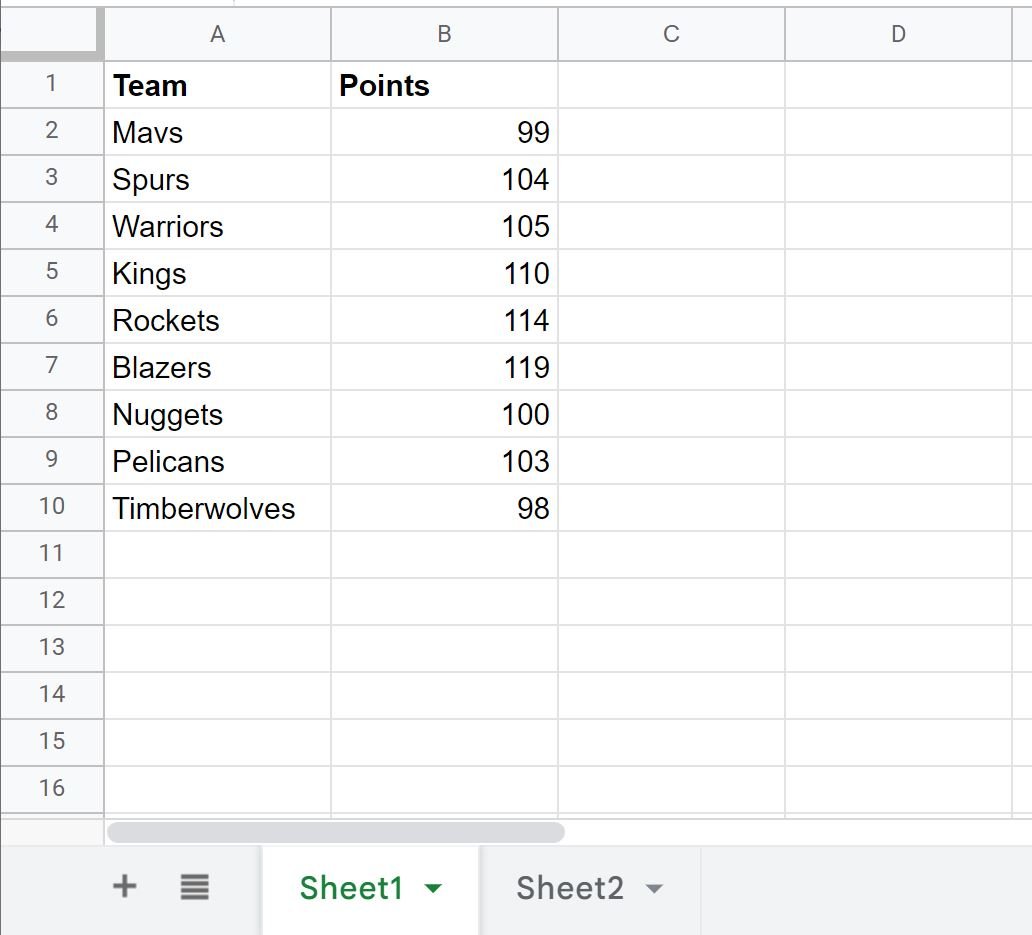
Suppose we have the following data in Sheet1 and Sheet2 in Google Sheets that contains information about various basketball teams:


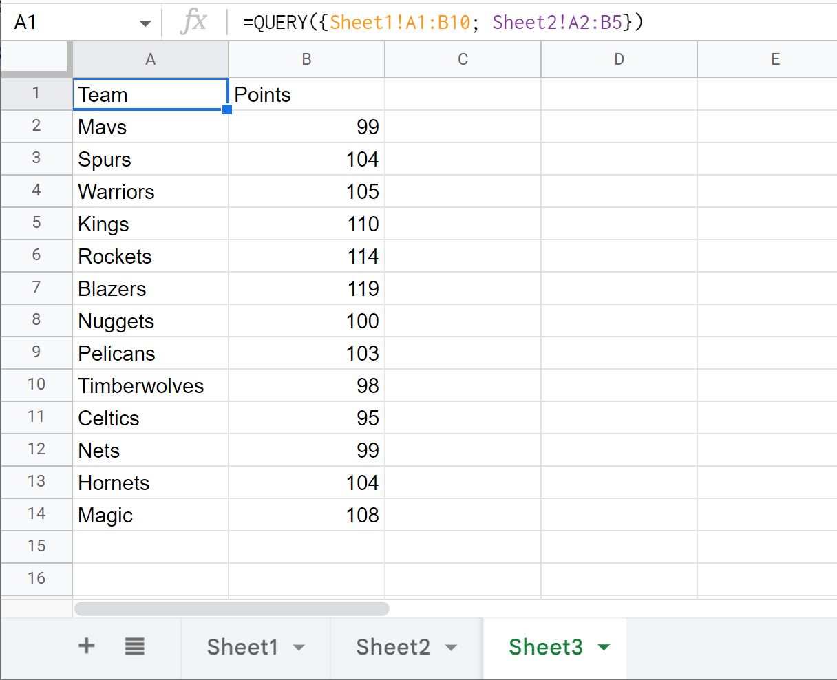
We can use the following formula to query data from both sheets and place the results in a new sheet called Sheet3:
=QUERY({Sheet1!A1:B10; Sheet2!A2:B5})
Here’s how to use the formula in practice:

Notice that the rows from Sheet1 are simply stacked on top of the rows from Sheet2.
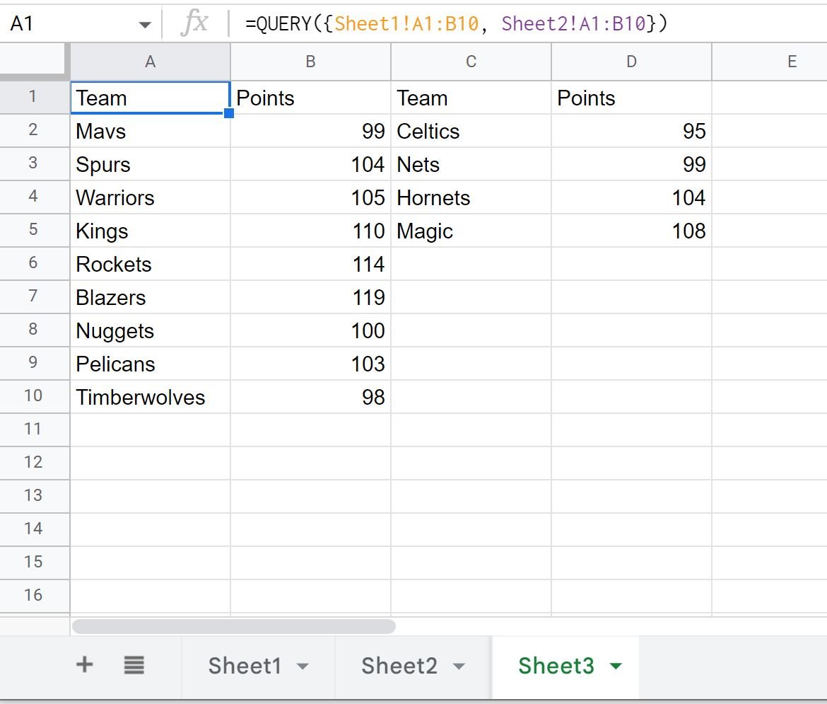
If you would instead like the rows from Sheet2 to be placed next to the rows from Sheet1, you can use a comma in the formula instead of a semi-colon:
=QUERY({Sheet1!A1:B10, Sheet2!A1:B10})
Here’s how to use the formula in practice:

Notice that the rows from Sheet2 are now placed next to the rows from Sheet1.
Note: In this example we only used two cell ranges, but you can use similar syntax to query from as many cell ranges as you’d like.
Additional Resources
The following tutorials explain how to perform other common queries in Google Sheets:
Google Sheets: How to Select Multiple Columns in Query
Google Sheets: How to Query From Another Sheet
Google Sheets: How to Use Group By in Query
Google Sheets: How to Use Order By in Query