Occasional you may want to find the top 10% of values in an Excel column. Fortunately there are two quick ways to do this:
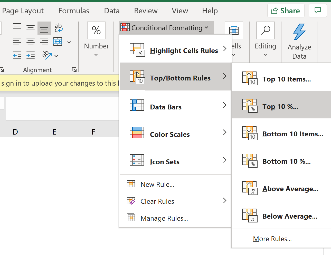
1. Use Conditional Formatting > Top/Bottom Rules > Top 10%
2. Filter using =CELL >=PERCENTILE(CELL RANGE, 0.9)
This tutorial provides an example of how to use each of these methods.
Example 1: Find Top 10% of Values Using Conditional Formatting
Suppose we have the following Excel column that contains 20 different values:
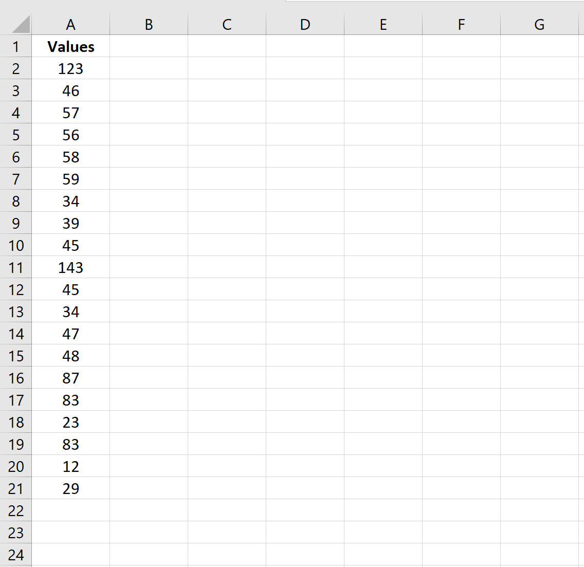
One way to find the top 10% of values in this column is to highlight all of the values in the column and then click Conditional Formatting > Top/Bottom Rules > Top 10%:
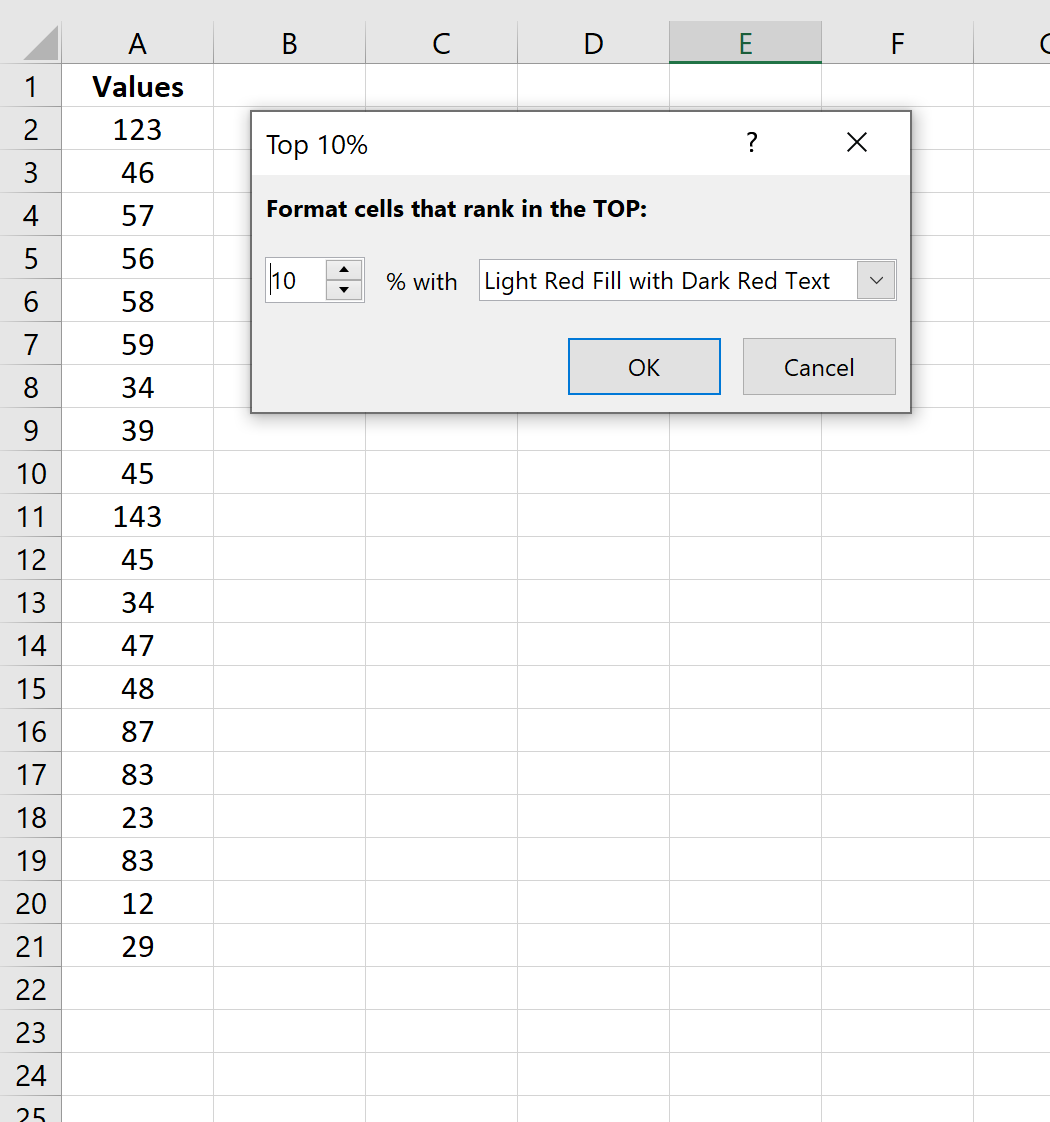
In the window that pops up, you’ll be given the option to highlight the top 10% of values using a certain color. We’ll leave it as the default option of light red with dark red text and click OK:
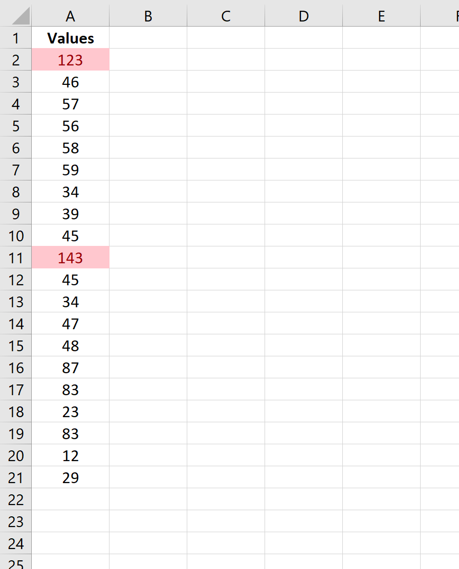
We can see that the values in the top 10% in this column are 123 and 143.
Example 2: Find Top 10% of Values Using a Formula
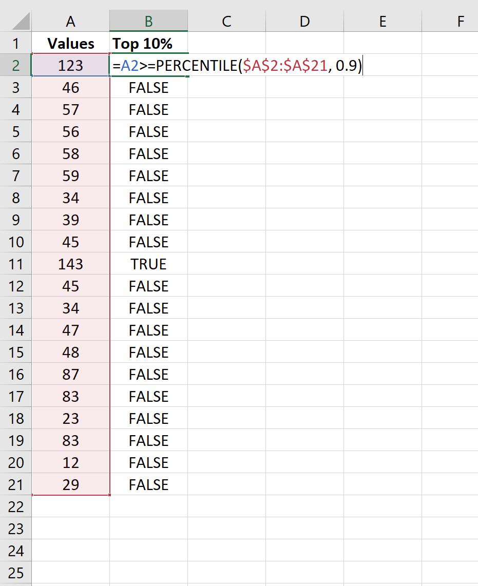
Another way to find the top 10% of values in a column is to create a new column of TRUE and FALSE values that indicate whether or not a given cell has a value at the 90th percentile or higher:
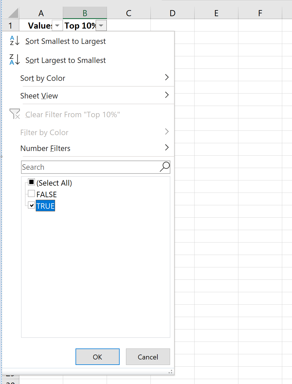
We can then click the Data tab along the top ribbon and click the Filter icon. We can then filter the Top 10% column to only show values that are TRUE:
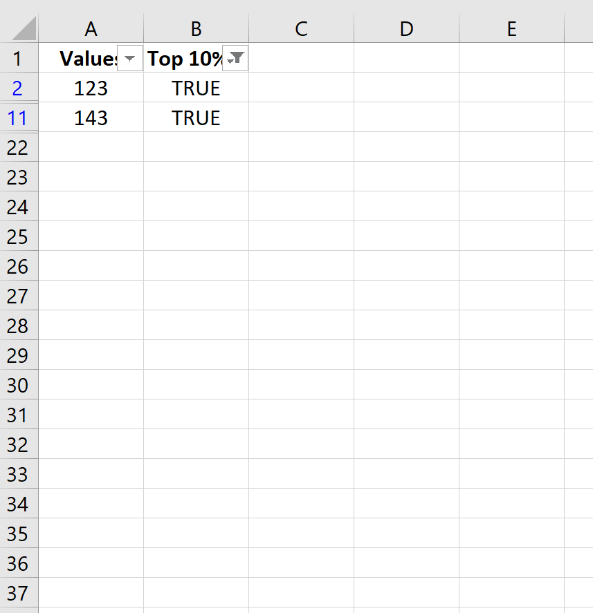
We can see that the values in the top 10% of all values are 123 and 143.
You can find more Excel tutorials here.